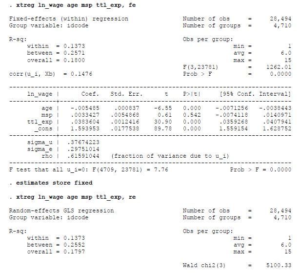
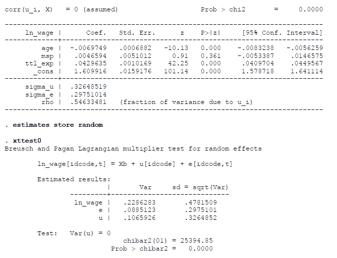
We model a relationship between wages (taken in natural logs!) and individual age (variable age, measured in years), marital status (msp=1, if a person has a spouse and 0 otherwise), work experience (variable ttl_exp, measured in years). We have estimated the fixed and random effects models and run some diagnostic tests.

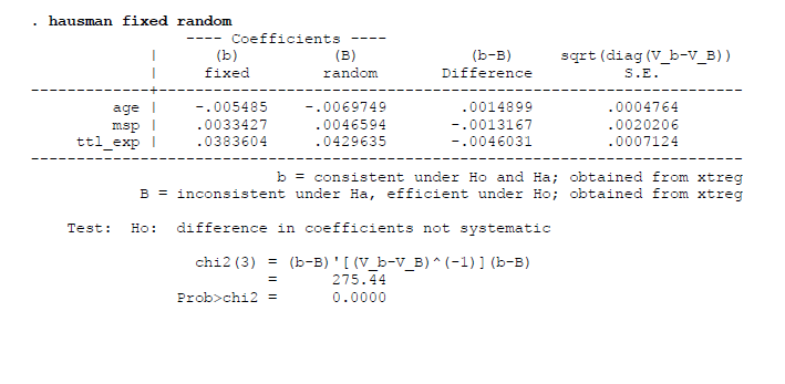
?) What do we actually check with the tests reported below - xttest0 ? hausman - and how should we interpret the results of these tests? Which model would you chose and why?

?) Should we (and if so, how?) interpret the coefficients on variables age, msp ? ttl_exp in the equation that you have chosen? What is the quantitative effect of these variables on wages?

. xtreg In wage age msp ttl exp, fe Fixed-effects (within) regression Number of obs 28, 494 11 1I Group variable: idcode Number of groups 4, 710 R-SQ : Obs per group: Within = 0.1373 min = 1 between = 0.2571 avg = 6.0 overall = 0.1800 max = 15 F (3, 23781) 1262 .01 corr (u_i, Xb) = 0.1476 Prob > F 0.0000 In wage I Coef. Std. Err. t PaltI [954 Conf. Interval] age - . 005485 . 000837 -6.55 0.000 - . 0071256 - . 0038443 msp . 0033427 . 0054868 0. 61 0. 542 - . 0074118 0140971 tt1 exp . 0383604 . 0012416 30.90 0. 000 . 0359268 . 0407941 cons 1. 593953 . 0177538 89.78 0.000 1 . 559154 1 . 628752 sigma_u 37674223 sigma_e . 29751014 rho | . 61591044 ( fraction of variance due to u_i) test that all u_i=0: F (4709, 23781) = 7.76 Prob > F = 0.0000 estimates store fixed xtreg In wage age msp ttl exp, re Random-effects GLS regression Number of obs = 28, 494 Group variable: idcode Number of groups = 4, 710 R-3q : Obs per group: within = 0.1373 min = 1 between = 0.2552 avg = 6.0 overall = 0.1797 max = 15 Wald chi2 (3) 5100.33corr (u i, x) = 0 (assumed) Prob > chi2 = 0 . 0000 In wage I Coef. Std. Err. Z P>Izl [95% Conf. Interval] age - . 0069749 . 0006882 -10.13 0. 000 -. 0083238 -. 0056259 msp . 0046594 . 0051012 0.91 0. 361 -. 0053387 . 0146575 tt1 exp . 0429635 . 0010169 42.25 0. 000 . 0409704 . 0449567 cons 1. 609916 . 0159176 101 .14 0.000 1. 578718 1 . 641114 sigma u | . 32648519 sigma e . 29751014 rho . 54633481 (fraction of variance due to u i) estimates store random xttest0 Breusch and Pagan Lagrangian multiplier test for random effects In_wage [idcode, t] = Xb + u[idcode] + e[idcode, t] Estimated results: Var sd = sqrt (Var) In wage .2286283 . 4781509 e . 0885123 . 2975101 . 1065926 . 3264852 Test: Var (u) = 0 chibar2 (01) = 25394.85 Prob > chibar2 = 0 . 0000. hausman fixed random --- Coefficients -- (b) (B) (b-B) sqrt (diag (V b-V B) ) fixed random Difference 5. E. age -. 005485 -. 0069749 . 0014899 . 0004764 msp . 0033427 . 0046594 -. 0013167 . 0020206 tt1 exp . 0383604 . 0429635 - . 0046031 . 0007124 b = consistent under Ho and Ha; obtained from xtreg B = inconsistent under Ha, efficient under Ho; obtained from xtreg Test: Ho : difference in coefficients not systematic chi2 (3) = (b-B) '[ (V b-V B) ~(-1)1 (b-B) 275.44 Prob>chi2 = 0. 0000