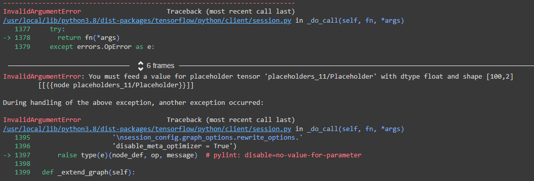
Question
When running the code below I am getting these errors. Any help fixing it would be appreciated. import numpy as np import tensorflow as tf
When running the code below I am getting these errors. Any help fixing it would be appreciated.

| import numpy as np
import tensorflow as tf
import matplotlib.pyplot as plt
tf.compat.v1.disable_eager_execution()
#1) Generate the synthetic data using the following Python code snippet.
# Generate synthetic data
N = 100
# Zeros form a Gaussian centered at (-1, -1)
x_zeros = np.random.multivariate_normal(mean=np.array((-1, -1)), cov=.1*np.eye(2), size=(N//2,))
y_zeros = np.zeros((N//2,))
# Ones form a Gaussian centered at (1, 1)
x_ones = np.random.multivariate_normal(mean=np.array((1, 1)), cov=.1*np.eye(2), size=(N//2,))
y_ones = np.ones((N//2,))
x_np = np.vstack([x_zeros, x_ones])
y_np = np.concatenate([y_zeros, y_ones])
# Plot x_zeros and x_ones on the same graph plt.scatter(x_zeros[:,0], x_zeros[:,1], label='class 0') plt.scatter(x_ones[:,0], x_ones[:,1], label='class 1') plt.legend() plt.show()
#3) Generate a TensorFlow graph.
with tf.name_scope("placeholders"):
x = tf.compat.v1.placeholder(tf.float32, (N, 2))
y = tf.compat.v1.placeholder(tf.float32, (N,))
with tf.name_scope("weights"):
W = tf.Variable(tf.random.normal((2, 1)))
b = tf.Variable(tf.random.normal((1,)))
with tf.name_scope("prediction"):
y_logit = tf.squeeze(tf.matmul(x, W) + b)
# the sigmoid gives the class probability of 1
y_one_prob = tf.sigmoid(y_logit)
# Rounding P(y=1) will give the correct prediction.
y_pred = tf.round(y_one_prob)
with tf.name_scope("loss"):
# Compute the cross-entropy term for each datapoint
entropy = tf.nn.sigmoid_cross_entropy_with_logits(logits=y_logit, labels=y)
# Sum all contributions
l = tf.reduce_sum(entropy)
with tf.name_scope("optim"):
train_op = tf.compat.v1.train.AdamOptimizer(.01).minimize(l)
with tf.name_scope("summaries"):
tf.compat.v1.summary.scalar("loss", l)
merged = tf.compat.v1.summary.merge_all()
train_writer = tf.compat.v1.summary.FileWriter('logistic-train', tf.compat.v1.get_default_graph())
#4) Train the model, get the weights, and make predictions.
with tf.compat.v1.Session() as sess: sess.run(tf.compat.v1.global_variables_initializer())
# Train model for i in range(1000): _, summary, loss = sess.run([train_op, merged, l], {x: x_np, y: y_np}) train_writer.add_summary(summary, i)
# Get weights and bias w_final, b_final = sess.run([W, b])
# Make predictions y_pred_np = sess.run(y_pred, {x: x_np})
train_writer.close()
#5) Plot the predicted outputs on top of the data.
x_min, x_max = x_np[:, 0].min() - .5, x_np[:, 0].max() + .5 y_min, y_max = x_np[:, 1].min() - .5, x_np[:, 1].max() + .5
xx, yy = np.meshgrid(np.linspace(x_min, x_max, 100), np.linspace(y_min, y_max, 100))
X_grid = np.c_[xx.ravel(), yy.ravel()]
with tf.compat.v1.Session() as sess: y_grid = sess.run(y_one_prob, {x: X_grid})
plt.contourf(xx, yy, y_grid.reshape(xx.shape), cmap=plt.cm.Paired) plt.scatter(x_np[y_np == 0, 0], x_np[y_np == 0, 1], c="red") plt.scatter(x_np[y_np == 1, 0], x_np[y_np == 1, 1], c="blue") plt.show() |
Step by Step Solution
There are 3 Steps involved in it
Step: 1

Get Instant Access to Expert-Tailored Solutions
See step-by-step solutions with expert insights and AI powered tools for academic success
Step: 2

Step: 3

Ace Your Homework with AI
Get the answers you need in no time with our AI-driven, step-by-step assistance
Get Started


