will give a great review
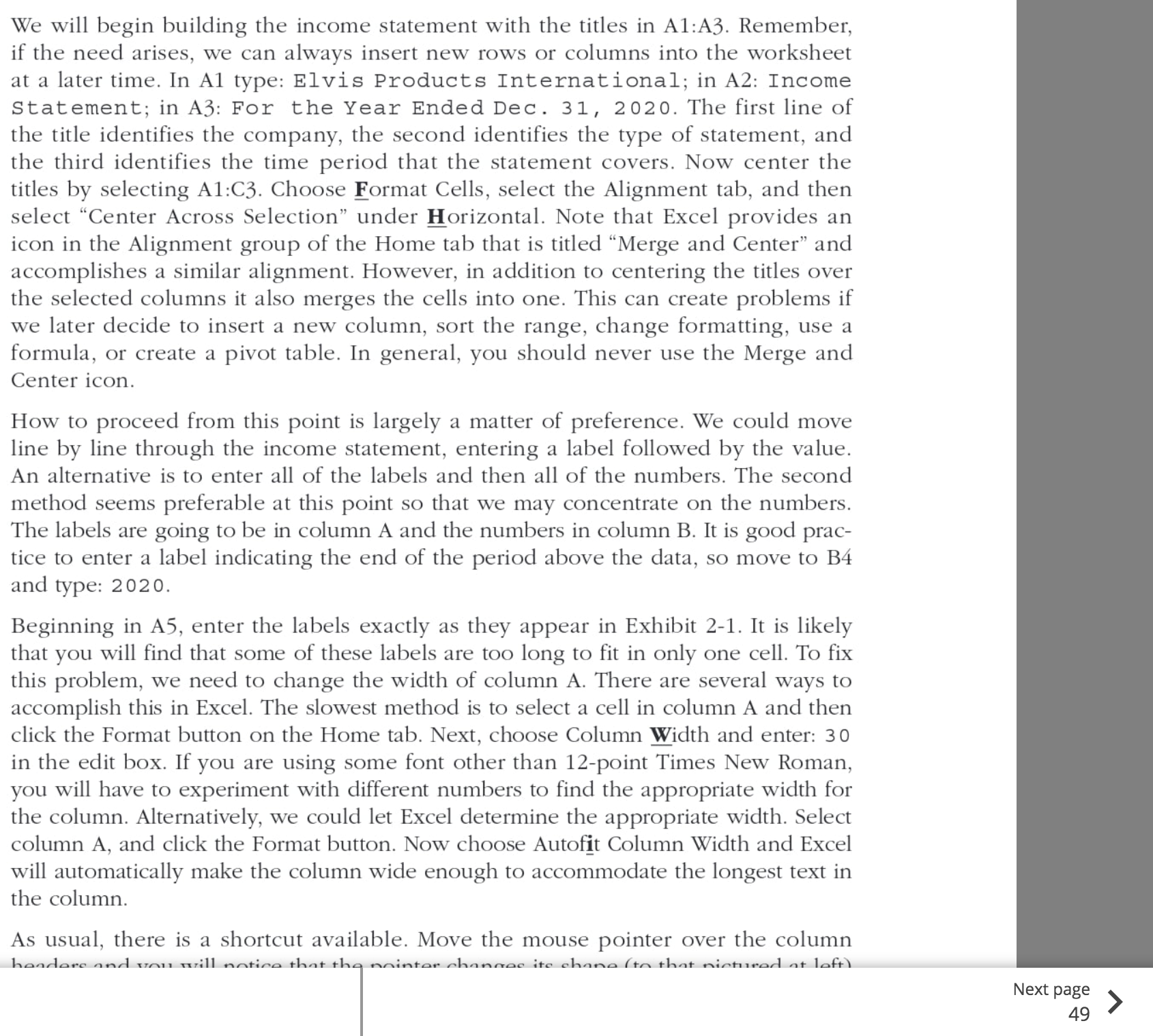
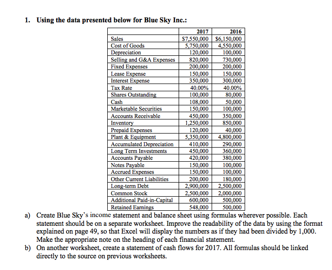
We will begin building the income statement with the titles in A1:A3. Remember, if the need arises, we can always insert new rows or columns into the worksheet at a later time. In A1 type: Elvis Products International; in A2: Income Statement; in A3: For the Year Ended Dec. 31, 2020. The first line of the title identifies the company, the second identifies the type of statement, and the third identifies the time period that the statement covers. Now center the titles by selecting A1:C3. Choose Eormat Cells, select the Alignment tab, and then select \"Center Across Selection\" under orizontal. Note that Excel provides an icon in the Alignment group of the Home tab that is titled \"Merge and Center\" and accomplishes a similar alignment. However, in addition to centering the titles over the selected columns it also merges the cells into one. This can create problems if we later decide to insert a new column, sort the range, change formatting, use a formula, or create a pivot table. In general, you should never use the Merge and Center icon. How to proceed from this point is largely a matter of preference. We could move line by line through the income statement, entering a label followed by the value. An alternative is to enter all of the labels and then all of the numbers. The second method seems preferable at this point so that we may concentrate on the numbers. The labels are going to be in column A and the numbers in column B. It is good prac- tice to enter a label indicating the end of the period above the data, so move to B4 and type: 2020. Beginning in A5, enter the labels exactly as they appear in Exhibit 2-1. It is likely that you will find that some of these labels are too long to fit in only one cell. To fix this problem, we need to change the width of column A. There are several ways to accomplish this in Excel. The slowest method is to select a cell in column A and then click the Format button on the Home tab. Next, choose Column Eidth and enter: 30 in the edit box. If you are using some font other than 12point Times New Roman, you will have to experiment with different numbers to find the appropriate width for the column. Alternatively, we could let Excel determine the appropriate width. Select column A, and click the Format button. Now choose Autofit Column Width and Excel will automatically make the column wide enough to accommodate the longest text in the column. As usual, there is a shortcut available. Move the mouse pointer over the column knnrlam apatl xtnil uti\" nnm that fl\" Mini-m nhnnnar.' I'fe 01"an (rn that rdnhannzl n:- lnFI-\\ Next page 49 > 1. Using the data presented below for Blue Sky Inc.: 2017 2016 Sales $7,550,000 $6,150,000 Cost of Goods 5,750,000 4,550.000 Depreciation 120,000 100,000 Selling and G&A Expenses 820,000 730,000 Fixed Expenses 200,000 200,000 Lease Expense 150,000 150,000 Interest Expense 350,000 300,000 Tax Rate 40.00% 40.00% Shares Outstanding 100,000 80,000 Cash 108,000 50.000 Marketable Securities 50,000 100,000 Accounts Receivable 450,000 350,000 Inventory 1,250,000 850,000 Prepaid Expenses 120,000 40.000 Plant & Equipment 5,350,000 4,800,000 Accumulated Depreciation 410,000 290,000 Long Term Investments 450,000 360,000 Accounts Payable 420,000 380,000 Notes Payable 50,000 100,000 Accrued Expenses 150,000 100,000 Other Current Liabilities 200,000 180,000 Long-term Debt 2,900,000 2,500,000 Common Stock 2,500,000 2,000,000 Additional Paid-in-Capital 600,000 500,000 Retained Earnings 548,000 500,000 a) Create Blue Sky's income statement and balance sheet using formulas wherever possible. Each statement should be on a separate worksheet. Improve the readability of the data by using the format explained on page 49, so that Excel will display the numbers as if they had been divided by 1,000. Make the appropriate note on the heading of each financial statement. b) On another worksheet, create a statement of cash flows for 2017. All formulas should be linked directly to the source on previous worksheets


