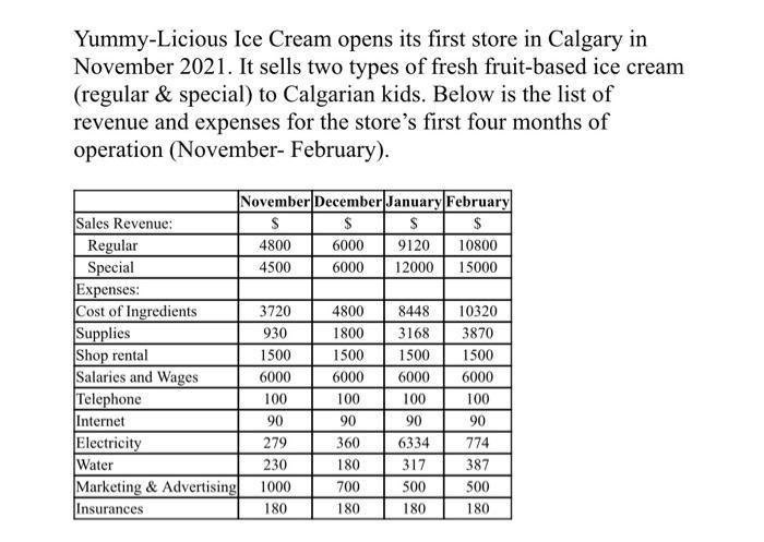
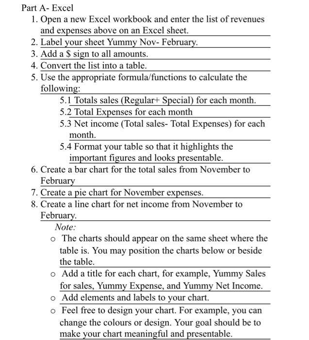
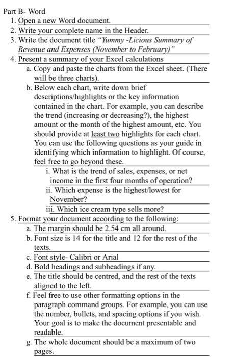
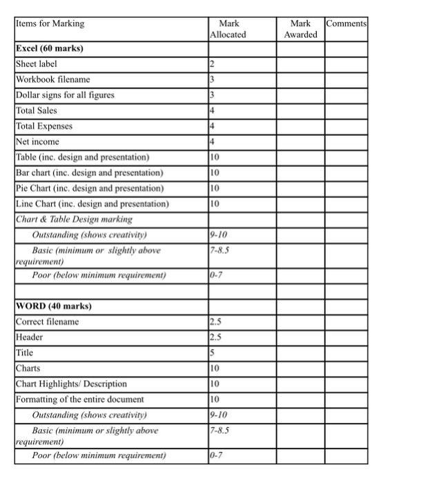
Yummy-Licious Ice Cream opens its first store in Calgary in November 2021. It sells two types of fresh fruit-based ice cream (regular & special) to Calgarian kids. Below is the list of revenue and expenses for the store's first four months of operation (November- February). Sales Revenue: Regular Special Expenses: Cost of Ingredients Supplies Shop rental Salaries and Wages Telephone Internet Electricity Water Marketing & Advertising Insurances November December January February $ S S $ 4800 6000 9120 10800 4500 6000 12000 15000 3720 930 1500 6000 100 90 279 230 1000 180 4800 1800 1500 6000 100 90 360 180 700 180 8448 10320 3168 3870 1500 1500 6000 6000 100 100 90 90 6334 774 317 387 500 500 180 180 Part A- Excel 1. Open a new Excel workbook and enter the list of revenues and expenses above on an Excel sheet. 2. Label your sheet Yummy Nov- February. 3. Add a $ sign to all amounts. 4. Convert the list into a table. 5. Use the appropriate formula/functions to calculate the following: 5.1 Totals sales (Regular+ Special) for each month. 5.2 Total Expenses for each month 5.3 Net income (Total sales- Total Expenses) for each month. 5.4 Format your table so that it highlights the important figures and looks presentable. 6. Create a bar chart for the total sales from November to February 7. Create a pie chart for November expenses. 8. Create a line chart for net income from November to February. Note: o The charts should appear on the same sheet where the table is. You may position the charts below or beside the table. o Add a title for each chart, for example, Yummy Sales for sales, Yummy Expense, and Yummy Net Income. o Add elements and labels to your chart. o Feel free to design your chart. For example, you can change the colours or design. Your goal should be to make your chart meaningful and presentable. Part B- Word 1. Open a new Word document. 2. Write your complete name in the Header. 3. Write the document title "Yummy -Licious Summary of Revenue and Expenses (November to February)" 4. Present a summary of your Excel calculations a. Copy and paste the charts from the Excel sheet. (There will be three charts). b. Below each chart, write down brief descriptions/highlights or the key information contained in the chart. For example, you can describe the trend (increasing or decreasing?), the highest amount or the month of the highest amount, etc. You should provide at least two highlights for each chart. You can use the following questions as your guide in identifying which information to highlight. Of course, feel free to go beyond these. i. What is the trend of sales, expenses, or net income in the first four months of operation? ii. Which expense is the highest/lowest for November? iii. Which ice cream type sells more? 5. Format your document according to the following: a. The margin should be 2.54 cm all around. b. Font size is 14 for the title and 12 for the rest of the texts. c. Font style- Calibri or Arial d. Bold headings and subheadings if any. e. The title should be centred, and the rest of the texts aligned to the left. f. Feel free to use other formatting options in the paragraph command groups. For example, you can use the number, bullets, and spacing options if you wish. Your goal is to make the document presentable and readable. g. The whole document should be a maximum of two pages. Items for Marking Excel (60 marks) Sheet label Workbook filename Dollar signs for all figures. Total Sales Total Expenses Net income Table (inc. design and presentation) Bar chart (inc. design and presentation) Pie Chart (inc, design and presentation) Line Chart (inc. design and presentation) Chart & Table Design marking Outstanding (shows creativity) Basic (minimum or slightly above requirement) Poor (below minimum requirement) WORD (40 marks) Correct filename Header Title Charts Chart Highlights/ Description Formatting of the entire document Outstanding (shows creativity) Basic (minimum or slightly above requirement) Poor (below minimum requirement) Mark Allocated 2 3 3 4 4 4 10 10 10 10 9-10 7-8.5 0-7 2.5 2.5 5 10 10 10 9-10 7-8.5 0-7 Mark Awarded Comments