Cases And Materials On Employment Law 8th Edition Richard Painter, Ann Holmes - Solutions

Discover comprehensive solutions for "Cases and Materials on Employment Law 8th Edition" by Richard Painter and Ann Holmes. Access the answers key and detailed solutions pdf for all chapters, providing step-by-step answers to solved problems. Enhance your understanding with our online solutions manual and instructor manual, designed to assist with textbook questions and answers. Our test bank offers chapter solutions and an array of questions and answers to aid your studies. Benefit from the free download of solutions, making it easier than ever to grasp complex employment law concepts.

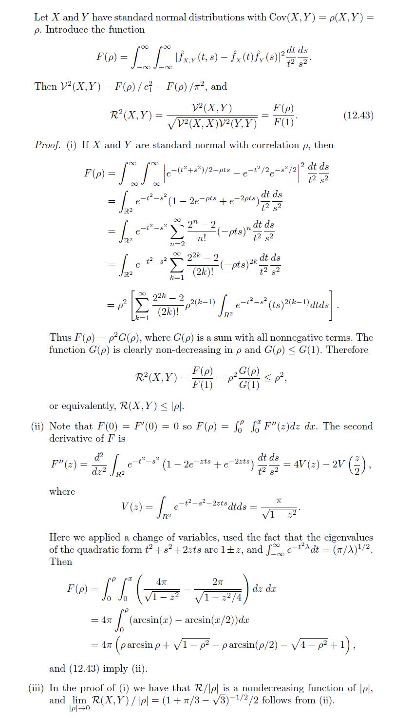
Refer to Exercise 19.4. Use hierarchical clustering to obtain a dendrogram graphical summary of the results as in Figure 4 of Székely and Rizzo [2013a]. Refer to the paper for details.Data From Exercise 19.4Exercise 19.4. Repeat Example 19.3 using the current 30 stocks of the Dow Jones Industrial
Give the detailed proofs of the four statements of Proposition 19.2 . Vz2(X, Y) R(X, Y)= V2(X,X) V(Y, Y)"
In the proof of Proposition 16.2 (unbiasedness of the inner product estimator of \(\mathcal{V}^{2}\) ) show that these formulas for expected values of \(T_{1}, T_{2}, T_{3}\) are correct:\[\begin{aligned}& E\left[T_{1}\right]=n(n-1) \gamma \\& E\left[T_{2}\right]=n(n-1)\{(n-2)(n-3) \alpha \beta+2
If \(E\left(|X|_{p}^{\alpha}+|Y|_{q}^{\alpha}\right)
Let \(\widehat{A}\) be a double-centered distance matrix. Prove or disprove the following statements:1. If \(B\) is the matrix obtained by double-centering \(\widehat{A}\), then \(B=\widehat{A}\).2. If \(c\) is a constant and \(B\) denotes the matrix obtained by adding \(c\) to the off-diagonal
Derive formula (12.26) for \(\mathcal{V}^{2}(X)\) if \(X\) has an exponential distribution with rate \(\lambda\). V(X) = (3X)1 = 0(X) 3
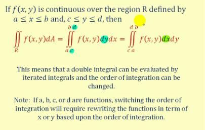
Prove Proposition 12.1. Apply Lemma 12.1 and Fubini's theorem. If f(x, y) is continuous over the region R defined by axband, c y d, then ba db ff f(x,y)dA = ff f(x, y)dx = f(x,y)dxdy R a This means that a double integral can be evaluated by iterated integrals and the order of integration can be
Prove that Wasserstein metric spaces are not of negative type.See Theorem 1.3 in Naor and Schechtman [2007]. It shows that Wasserstein does not have isometric embeddings into Hilbert spaces.
In the goodness-of-fit test procedure of Section 4.5, instead of the estimated critical value cαcα, give a formula for a an estimated pp-value. Source code of the energy goodness-of-fit test functions.
Extend Lemma 3.1 (Lemma 2.1) for \(\alpha otin(0,2)\). In particular, is it true that for \(-d
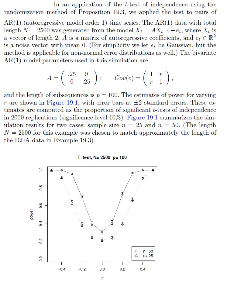
Replicate the results of Example 19.2 using the same simulation design. In an application of the t-test of independence using the randomization method of Proposition 19.3, we applied the test to pairs of AR(1) (autoregressive model order 1) time series. The AR(1) data with total length N = 2500 was
Derive formulas (5.27) and (5.28). Exi X = 4x(xi) + 40(xi) 3xi + -
Derive formula (12.24) for \(\mathcal{V}^{2}(X)\) if \(X\) has a \(\operatorname{Gaussian}(\mu, \sigma)\) distribution. See the proof of Theorem 12.4. V(X)=1[+] 0(X). 4[ 1-3
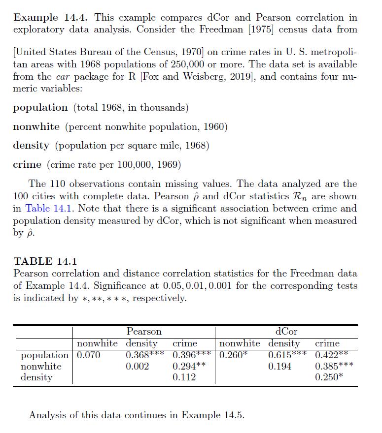
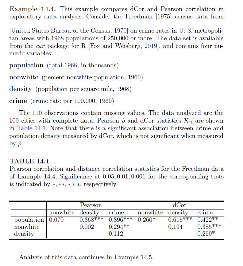
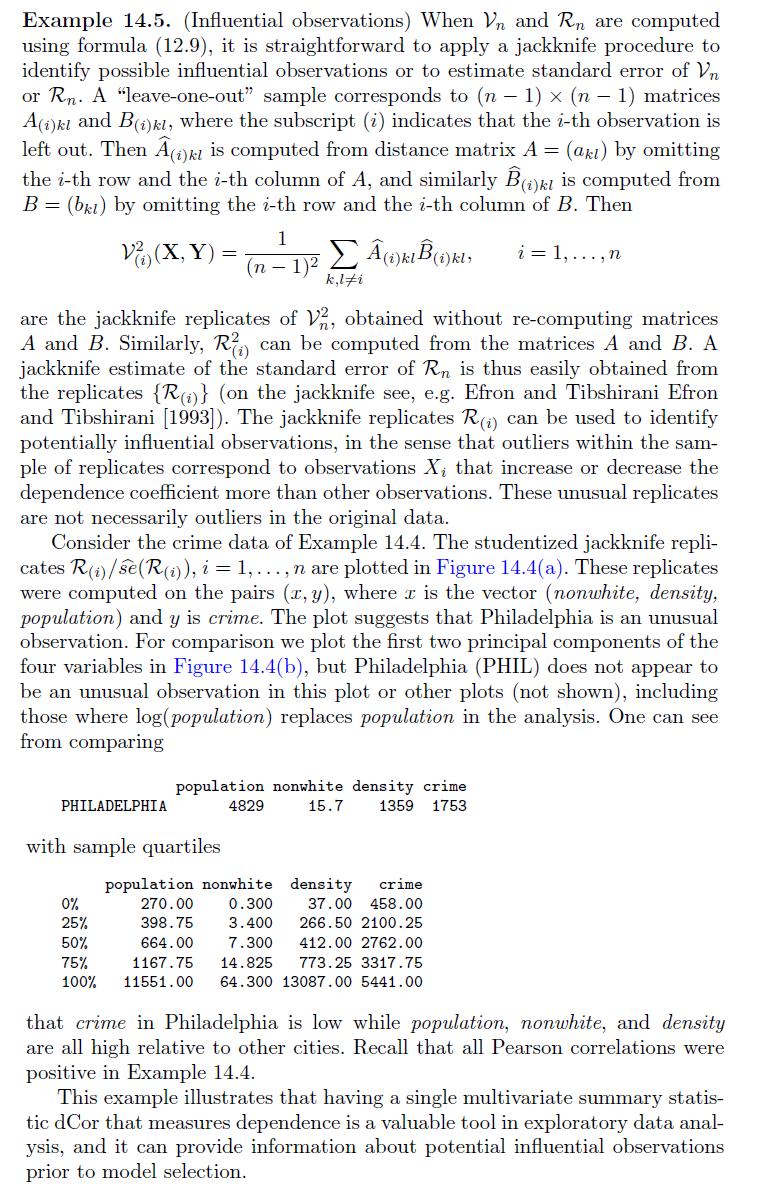
Let \(\mathbf{X}\) be a sample \(\left\{X_{1}, \ldots, X_{n}ight\}\), and let \(A=\left(a_{i j}ight)\) be the matrix of pairwise Euclidean distances \(a_{i j}=\left|X_{i}-X_{j}ight|\). Suppose that \(\pi\) is a permutation of the integers \(\{1, \ldots, n\}\). In a permutation test we re-index one
Repeat Examples 14.4 and 14.5 on the crime data. Example 14.4. This example compares dCor and Pearson correlation in exploratory data analysis. Consider the Freedman [1975] census data from [United States Bureau of the Census, 1970] on crime rates in U. S. metropoli- tan areas with 1968 populations
Prove that\[\begin{aligned}& (E[(X-E(X))(Y-E(Y))])^{2} \\& \quad=E\left[(X-E(X))\left(X^{\prime}-E\left(X^{\prime}ight)ight)(Y-E(Y))\left(Y^{\prime}-E\left(Y^{\prime}ight)ight)ight]\end{aligned}\]
Which of the properties of dCov and dCor \((\alpha=1)\) in Section 12.5 hold for arbitrary exponents \(0
Discuss the result if in the definition of Brownian distance covariance, Brownian motion is replaced by other stochastic processes like the Poisson process or pseudorandom processes. For the definition of a pseudorandom process see Móri and Székely [2022].
It is obvious that \(\widetilde{A}=0\) if all sample observations are identical. More generally, show that \(\widetilde{A}=0\) if and only if the \(n\) sample observations are equally distant or at least \(n-1\) of the \(n\) sample observations are identical.
Let \(\theta=\operatorname{Cov}(X, Y)\) and consider the sample covariance statistic\[S_{X Y}=\frac{1}{n-1} \sum_{i=1}^{n}\left(X_{i}-\bar{X}ight)\left(Y_{i}-\bar{Y}ight)\]Show that \(S_{X Y}\) is a U-statistic for \(\sigma_{X Y}=\operatorname{Cov}(X, Y)\) What is the kernel function?
Suppose that XX is a sample, Extra \left or missing ightExtra \left or missing ight is the distance matrix of the sample, ˆAA^ is the double-centered distance matrix and ˜AA~ is the U-centered distance matrix of the sample.(a) State and prove necessary and sufficient conditions that ˆAA^ is the
Prove statements (i), (ii), and (iii) of Lemma 17.1. Lemma 17.1. Let A be a U-centered distance matrix. Then 1. Rows and columns of A sum to zero. 2. (A) = . That is, if B is the matrix obtained by U-centering an element A. A Hn, B = A. 3. A is invariant to double centering. That is, if B is the
Show that the corrected double-centered distance matrices \(A^{*}=\left(A_{i j}^{*}ight)\) defined in (19.6) have the property that \(E\left[A_{i, j}^{*}ight]=0\) for all \(i, j\). A1.j ={ = (Aijaij), n1 (ai -), n n n i j; i = j, Bij = n1(Bij-bi), n1 (bi - b), i j; i = j.
Repeat Example 19.3 using the current 30 stocks of the Dow Jones Industrial Average and the daily returns for the most recent 10 years. (Historical stock price data is available online; in particular, adjusted closing prices can be downloaded from the Yahoo! finance site.) Example 19.3 (Dow Jones
Which of the dependence measures discussed in the examples satisfy Axiom (i)? Justify the answers with proofs or counterexamples.
Prove that an alternate computing formula for \(\mathrm{dCor}_{n}^{2}\) (Definitions \(12.5-12.7)\) is\[\mathrm{dCor}_{n}^{2}(X, Y)=\frac{\left\langle C \Delta_{X} C, C \Delta_{Y} Cightangle}{\left\|C \Delta_{X} Cight\|\left\|C \Delta_{Y} Cight\|}\]where \(\Delta_{X}, \Delta_{Y}\) are the Euclidean
Prove by constructing an example that a monotone invariant \(\Delta\) can satisfy Axioms (i) - (iv). One idea is to apply distance correlation to the ranks of observations (or to the copula). Are there also homeomorphism invariant versions? (They are invariant with respect to all continuous 1-1
Prove by constructing an example that maximal correlation can be 1 for uncorrelated random variables.
In Example 2.1, if the null hypothesis is true, \(F_{X}=F_{0}\). Thus, \(\mathcal{E}(X, Y)=2 E|X-Y|-E\left|X-X^{\prime}ight|-E\left|Y-Y^{\prime}ight|=0\). Show that for the \(U\)-statistic, \(E\left(\mathcal{E}_{n}^{*}ight)=0\). That is, show that the \(U\)-statistic given by (2.3) is unbiased for
In Example 2.2, if \(X, Y\) are independent and \(F_{X}=F_{Y}\) then \(\mathcal{E}(X, Y)=2 E|X-Y|-E\left|X-X^{\prime}ight|-E\left|Y-Y^{\prime}ight|=0\). However, the test statistic \(\frac{n m}{n+m} V_{n, m}=\frac{n m}{n+m} \mathcal{E}_{n, m}\) is not unbiased for \(\mathcal{E}(X, Y)\). Show that
For the two-sample energy statistic, prove that under the null hypothesis \(H_{0}: X \stackrel{D}{=} Y\), the expected value of the test statistic \(\frac{n m}{n+m} \mathcal{E}_{n, m}(\mathbf{X}, \mathbf{Y})\) is \(E|X-Y|\).
Prove that the two-sample energy test for equal distributions is consistent. Hint: Prove that under an alternative hypothesis,\[E\left[\frac{n m}{n+m} \mathcal{E}_{n, m}(\mathbf{X}, \mathbf{Y})ight]>\frac{n m}{n+m} \mathcal{E}(X, Y)\]
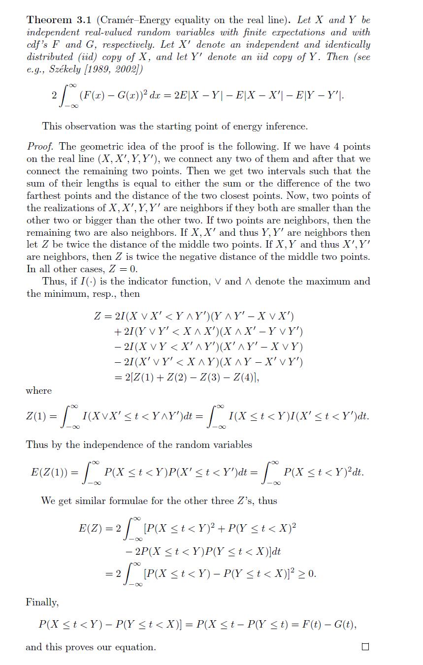
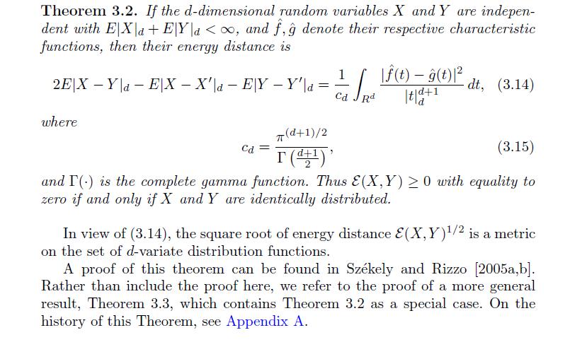
Refer to the energy goodness-of-fit test of the two-parameter exponential family \(T \sim \operatorname{Exp}(\mu, \lambda)\) described in Section 3.1. Prove that under the null hypothesis, the expected distances are\[\begin{aligned}& E|t-T|=t-\mu+\frac{1}{\lambda}\left(1-2 F_{T}(t)ight), \quad t
Using Theorem 3.2 and equation (3.13) give another proof for the Cramér-Energy equality on the real line (Theorem 3.1).If \(d=1\) then \(c_{d}=c_{1}=\pi\) and thus if we compare the left-hand sides of (3.13) and Theorem 3.1 we get\[2 \int_{-\infty}^{\infty}(F(x)-G(x))^{2} d x=\mathcal{E}(X,
Using software, check that formula (3.9) holds for a numerical example, say aircondit data in the boot package or other small data set. If using \(R\), see \(R\) functions sort, seq, and dist. n n |X - X,| = 2((2k 1) n)() i,j=1 k=1
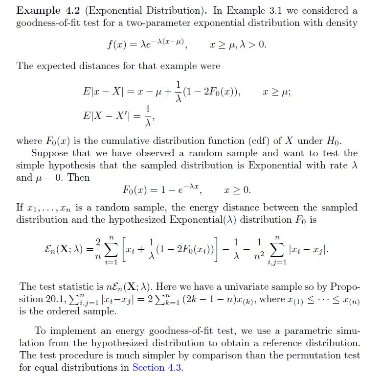
Implement a goodness-of-fit test for the Exponential distribution (see Example 4.2) in R. See the help topics for rexp (random exponential generator), dist (Euclidean distances) and replicate (utility to construct the loop for the replicates).Example 4.2 Example 4.2 (Exponential Distribution). In
Derive formula (4.4) for the expected distance E|x−X|E|x−X| if XX is Normal(μ,σ2)Normal⁡(μ,σ2). Write the integrals in the expression as F(x)F(x) or 1−F(x)1−F(x). E|x X| = 2(x )F(x) +20 f(x) (x ), - -
Derive equation (5.7). That is, prove that if \(0\[E|y-X|=2 y F(y)-y+\frac{\alpha}{\alpha+\beta}-2 \frac{B(\alpha+1, \beta)}{B(\alpha, \beta)} G(y),\]where \(G\) is the \(\operatorname{CDF}\) of \(\operatorname{Beta}(\alpha+1, \beta)\). E|X X'| = 2e-2 [Io (2X) + I1(2X)].
Do a small power study to investigate whether the Poisson M-test and the energy test (E-test) have different power performance. Some alternatives to consider could be Poisson mixtures (different \(\lambda\) ), negative binomial, zero-modified or zero-inflated Poisson, or other counting
Run a benchmark comparison to compare the running times of the Poisson M-test and E-test. Is there a noticeable difference? The microbenchmark package for \(\mathrm{R}\) is convenient for this [Mersmann, 2021].
Write an \(\mathrm{R}\) function to compute the energy test statistic for a goodness-of-fit test of the simple hypothesis \(H_{0}: X \sim \operatorname{Beta}(\alpha, \beta)\), where \(\alpha, \beta\) are specified. How would you modify the function for the composite hypothesis?
Prove that if \(Z_{1}, Z_{2}, \ldots Z_{n}\) are \(d\)-dimensional iid standard normal random variables,\[\bar{Z}=\frac{1}{n} \sum_{i=1}^{n} Z_{i}, \quad S_{n}=\frac{1}{n-1} \sum_{i=1}^{n}\left(Z_{i}-\bar{Z}ight)\left(Z_{i}-\bar{Z}ight)^{T}\]and \(Y_{i}=S_{n}^{-1 / 2}\left(Z_{i}-\bar{Z}ight),
Prove that under the hypothesis of normality for every fixed integer \(d \geq 1\),1. \(E\left[\widehat{\mathcal{E}}_{n, d}ight]\) is bounded above by a finite constant that depends only on \(d\).2. For every fixed \(\alpha \in(0,1)\), the sequence of critical values \(c_{\alpha, n, d}\) of
Solve Schrödinger equation (7.6) for \(f(x)=\frac{1}{2}\) on \([-1,1]\), when \(\psi^{\prime}(-1)=\psi^{\prime}(1)=0\). 1 2f " = .
Prove that if \(X\) is symmetric stable and \(E|x-X|^{s}
Yang [2012] computes \(E|x-X|^{s}\) as \(|x|^{s}\) for \(|x| \geq 2000\). Compute the relative error in this approximation. That is, compute (true value approximate value)/(true value) for the Cauchy distribution when \(x=2000\).
Prove that if \(X\) is \(d\)-dimensional standard normal, then\[\lim _{|x|_{d} ightarrow \infty} \frac{E|x-X|_{d}}{|x|_{d}} ightarrow 1\]
Prove that in the univariate case, with \(\alpha=2\), the disco decomposition is the ANOVA decomposition of variance. Start by finding an identity between SST and \(S_{2}\).
Prove Theorem 9.2. Theorem 9.2 (Li [2015a]). Suppose that P= {1, 2,...} is a partition of the data, and Pa = {, ,..., k} is the partition obtained by moving point a from to 2. Then Wa(P) - Wa(Pa) = = n1 2(1) n2 Ea (a, ) 2(n + 1) -Ea(a, ), (9.11) where Ea(a, Ti) denotes the two-sample a-energy
Show that the update formula of \(k\)-groups and Hartigan and Wong's \(k\)-means algorithm are the same when \(\alpha=2\).
Prove that a metric space \((X, d)\) has strong negative type if and only if the space of probability measures on \((X, d)\) equipped with the energy distance \(D\) has strong negative type.According to Schoenberg [1937] and Schoenberg [1938b] \((X, d)\) is of negative type iff there is a Hilbert
There are many widely used classical distances like the Hausdorff distance between non-empty compact subsets of a set in a metric space \((M, d)\) or the Fréchet distance between continuous curves. Do they have (strong) negative type?
(i) Show that variograms defined for real-valued stochastic processes or for random fields \(Z(x), x \in X\) as twice \(\operatorname{Var}\left[Z\left(x_{1}ight)-Z\left(x_{2}ight)ight], x_{1} \in \mathcal{X}, x_{2} \in \mathcal{X}\), are conditionally negative definite.Suppose the expected values
Show that \(\mathrm{d} \operatorname{Cor}(X, Y)\) is scale invariant.
Show that the double-centered distance matrix \(\hat{A}\) of Definition 12.4 has the property that each of the row and column means of \(\hat{A}\) are equal to zero.
Prove that \(\mathcal{V}_{n}(\mathbf{X})=0\) implies that all sample observations of \(\mathbf{X}\) are identical.
Prove that if \(\mathbf{X}\) is an \(n \times p\) data matrix, then \(\operatorname{dVar}_{n}(a+\) \(b \mathbf{X} C)=|b| \operatorname{dar}_{n}(\mathbf{X})\), for all constant vectors \(a\) in \(\mathbb{R}^{p}\), scalars \(b\), and \(p \times p\) orthonormal matrices \(C\).
Is it true that \(\operatorname{Cov}\left(\left|X-X^{\prime}ight|,\left|Y-Y^{\prime}ight|ight)=0\) implies that \(X\) and \(Y\) are independent? (Recall that \(X, X^{\prime}\) are iid; \(Y, Y^{\prime}\) are iid.)It is not hard to show that the following example is a counterexample. Define the
Does the independence of \(X-X^{\prime}\) and \(Y-Y^{\prime}\) imply the independence of \(X\) and \(Y\) ?
Derive formula (12.25) for \(\mathcal{V}^{2}(X)\) if \(X\) has the continuous uniform distribution on \([a, b]\). v(X) = 21b-a = 24/0 (X). 45
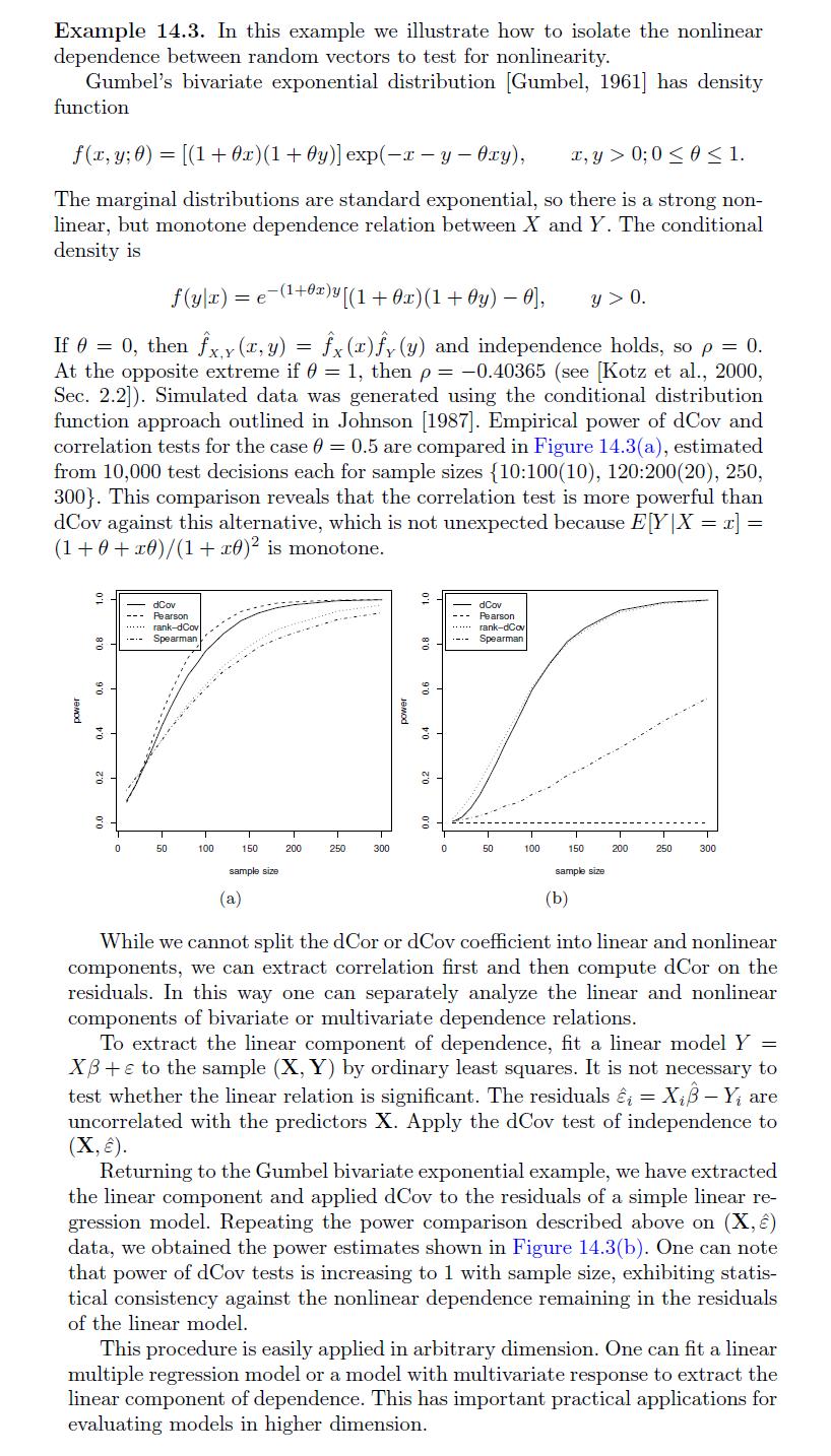
Implement the study in Example 14.3 and compare your results to the example. Example 14.3. In this example we illustrate how to isolate the nonlinear dependence between random vectors to test for nonlinearity. Gumbel's bivariate exponential distribution [Gumbel, 1961] has density function f(x, y;
Repeat Examples 14.4 and 14.5 on some other available data set in any R package or other source. Example 14.4. This example compares dCor and Pearson correlation in exploratory data analysis. Consider the Freedman [1975] census data from [United States Bureau of the Census, 1970] on crime rates in
From Lemma 17.1(iv), U-centered distance matrices have an additive constant invariance property. Show that this invariance property does not hold for double-centered distance matrices.Lemma 17.1 4. If c is a constant and B denotes the matrix obtained by adding c to the off-diagonal elements of A,

Cases And Materials On Employment Law 8th Edition Richard Painter, Ann Holmes - Solutions

Step by Step Answers