Curvilinear Polynomial Regression In this section we studied multiple linear regression. Our basic linear model has been y 5b0 1b1x1 1b2x2 1 1bk xk .

Since all the variables x1, x2 , …, xk are of first degree, this is an example of linear regression.

However, the same basic methods of linear regression can be used for curvilinear regression (also known as polynomial regression). The interested reader can find a great deal of information on this topic in the book Applied Numerical Methods by Carnahan, Luther, and Wilkes.

Assume we have at least k 1 2 data pairs (x, y)

and we want to approximate y using a polynomial of degree k. To do this, we make the following identification.

x x x x x x xk x 5 ; 5 ; 5 ; …; 5 k.

Then we use our known methods of multiple regression to obtain coefficients b0 , b1, b2 , b3 , …, bk and the equation 5 0 1 1 1 2 1 1 1 2 3 y b b x b x b x3 b x k k .
This is called the least-squares curvilinear regression model.
Marketing studies show that price increases often have a point of diminishing returns. For a popular product, the price can often increase with sales. However, when the price becomes too high, sales start to drop off. In the following graph, P 5point of diminishing returns.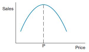

To estimate the point of diminishing returns, we use a quadratic polynomial, y 5b0 1b1x 1b2x 2. A very popular women’s knit T-shirt was tested for sales appeal and price in six large department stores. In each city, the T-shirts were advertised extensively in the local media, so price and sales initially went up. However, as price increased, sales eventually dropped off. Let x 5price per T-shirt in dollars and y 5number of T-shirts sold in a day at that price. We have the following data.

City A B C D E F x 12.97 13.88 15.95 18.50 19.99 22.50 y 23 31 33 29 25 17 To construct our quadratic polynomial, we use multilinear regression with the following table of data values.
x1 5 x 12.97 13.88 15.95 18.50 19.99 22.50 2 5 x x2 168.22 192.65 254.40 342.25 399.60 506.25 y 23 31 33 29 25 17 Computer software gives us coefficients for the model y 5b0 1b1x1 1b2x2 5b0 1b1x 1b2x 2, which becomes y 5293.80 115.10x 2 0.45x2.
The coefficient of determination is r2 5 0.88 (not too bad!). The curvilinear regression equation y 5293.80 115.10x 2 0.45x2 is a quadratic curve that opens downward. A little extra mathematics shows that the top point on the curve (point of diminishing returns) occurs when the cost per shirt of x 5$16.78 with y 5 32.87 shirts sold per day. This suggests the knit T-shirts should be priced at $16.78 and that about 33 of them will sell per day in a large department store.
Use the Internet, school library, popular magazines, or any other source to collect (x, y) data pairs regarding variables of interest to you. Construct a curvilinear regression model from your data and interpret the results.AppendixLO1

Transcribed Image Text:

Sales | P Price