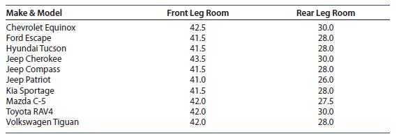
(Scatterplots, Correlation, and the Regression Line) The data from Example 2.17 give the front and rear leg rooms (in inches) for 10 different compact sports utility vehicles

1. Enter the data from columns 2 and 3 into L1 and L2. The scatterplot is created using 2nd ➤ stat plot, choosing Plot1 and the first type (Scatterplot). Lists L1 and L2 are the default settings for the x and y variables, but you can change the list numbers if you need to. Press zoom ➤ 9 (or ZoomStat) to display the scatterplot (Figure 3.19).

2. So that your calculator can display the value for r, press 2nd ➤ catalog. Scroll down to find DiagnosticOn and press enter twice. To find the correlation coefficient and the regression line, use stat ➤ CALC ➤ LinReg(a1bx) (the 8th entry in the list) and press enter. On the screen that appears (TI-84), the default Lists are L1 and L2. Scroll down to Store RegEQ and press vars ➤ Y-VARS ➤ Function ➤ Y1 ➤ enter (this stores the equation of the regression line in the Y-editor) (Figure 3.20(a)). When you move your cursor down to the word Calculate and press enter, the values for

a, b, r will appear (Figure 3.20(b)). For the TI-83, use stat ➤ CALC ➤ LinReg(a1bx), followed by L1, L2, Y1 and press enter twice. You can see the equation of the regression line by pressing y 5 and can plot the line on the scatterplot using zoom ➤ 9 (or ZoomStat). The trace command will allow you to see the equation of the line and the various data points (Figure 3.20(c)).

Transcribed Image Text:

Make & Model Chevrolet Equinox Ford Escape Hyundai Tucson Jeep Cherokee Jeep Compass Jeep Patriot Kia Sportage Front Leg Room Rear Leg Room 42.5 30.0 41.5 28.0 41.5 28.0 43.5 30.0 41.5 28.0 41.0 26.0 41.5 28.0 Mazda C-5 42.0 27.5 Toyota RAV4 42.0 30.0 Volkswagen Tiguan 42.0 28.0