In Section 20.6.1, MPC was applied to the Wood-Berry distillation column model. A MATLAB program for this example and constrained MPC are shown in Table E20.9.

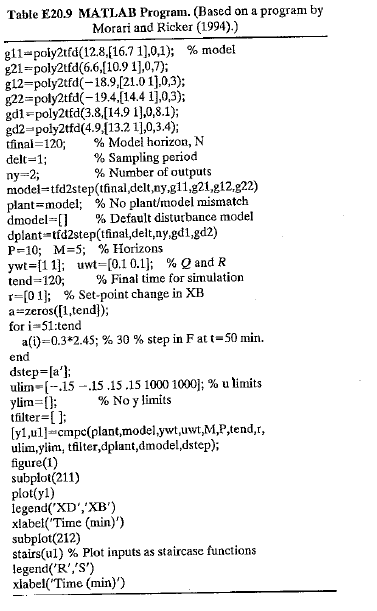
The design parameters have the base case values (Case B in Fig.) except for P =10 and M = 5. The input constraints are the saturation limits for each input (-0.15 and +0.15). Evaluate the effects of control horizon M and input weighting matrix R by simulating the Set-point change and the first disturbance of Section 20.6.1 for the following parameter values:

(a) Control horizon, M = 2 and 5

(b) Input weighting matrix, R = 0.1I and R = I

Consider plots of both inputs and outputs. Which choices of M and B provide the best control? Do any of these MPC controllers provide significantly better control than the controllers shown in Figs. 20.13 and 20.14? Justify your answer.

Table E20.9 MATLAB Program. (Based on a program by Morari and Ricker (1994).) gl1-poly2tfd(12.8(16.7 1),0,1); % model g21=poly2tfd(6.6,[10.9 1],0,7); g12-poly2tfd(-18.9,[21.0 1].0,3); g22=poly2tfd(-19.4.[14.4 1],0,3); gd1-poly2tfd(3.8,[14.9 1),0,8.1); gd2-poly2tfd(4.9.{13.2 1],0,3.4); tfinal=120; delt=1; % Model horizon, N % Sampling period % Number of outputs ny=2; model=tfd2step(tfinal,delt,ny,g11,g21,g12.g22) plant=model; % No plant/model mismatch dmodel=[] dplant=tfd2step(tfinal,delt,ny.gd1,gd2) P=10; M=5; % Horizons ywt=[1 1]; uwt=[0.1 0.1); % Q and R tend=120; % Default disturbance model %3D % Final time for simulation r=[0 1); % Set-point change in XB a=zeros([1,tend}); for i-51:tend a(i)=0.3*2.45; % 30 % step in F at t= 50 min. end dstep=[a'): ulim=(-.15 -.15.15.15 1000 1000]; % u limits ylim=[]; tfilter=[ ]; [y1,ul]=cmpc(plant,model,ywt,uwt,M,P,tend,r, ulim,ylin, tfilter, dplant,dmodel,dstep); figure(1) subplot(211) plot(yl) legend('XD','XB') xlabel('Time (min)') subplot(212) stairs(ul) % Plot inputs as staircase functions legend('R','S') xlabel("Time (min)') % No y limits