The Porsche Club of America sponsors driver education events that provide high-performance driving instruction on actual race tracks. Because safety is a primary consideration at such events, many owners elect to install roll bars in their cars. Deegan Industries manufactures two types of roll bars for Porsches. Model DRB is bolted to the car using existing holes in the car€™s frame. Model DRW is a heavier roll bar that must be welded to the car€™s frame. Model DRB requires 20 pounds of a special high alloy steel, 40 minutes of manufacturing time, and 60 minutes of assembly time. Model DRW requires 25 pounds of the special high alloy steel, 100 minutes of manufacturing time, and 40 minutes of assembly time. Deegan€™s steel supplier indicated that at most 40,000 pounds of the high-alloy steel will be available next quarter. In addition, Deegan estimates that 2000 hours of manufacturing time and 1600 hours of assembly time will be available next quarter. The profit contributions

$200 per unit for model DRB and $280 per unit for model DRW. The linear programming model for this problem is as follows:

Max 200 DRB + 280DRW

s.t.

20DRB + 25DRW ‰¤ 40,000 Steel available

40DRB + 100DRW ‰¤ Manufacturing minutes

60DRB + 40DRW ‰¤ 96,000 Assembly minutes

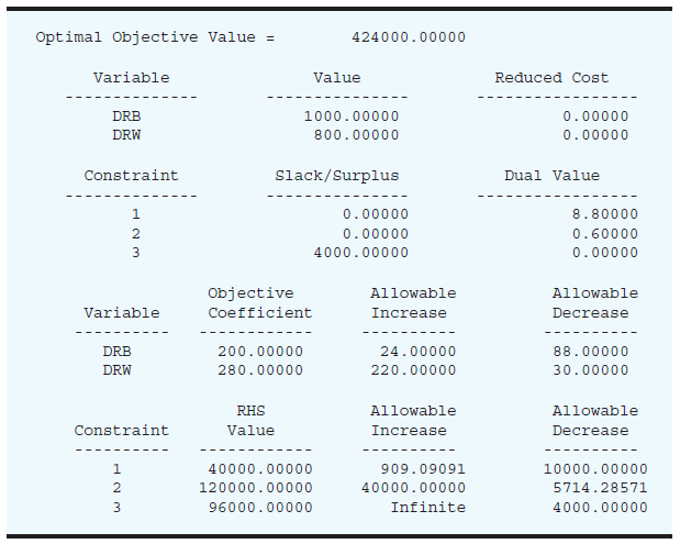
The computer solution is shown in Figure 3.20.

a. What are the optimal solution and the total profit contribution?

b. Another supplier offered to provide Deegan Industries with an additional 500 pounds of the steel alloy at $2 per pound. Should Deegan purchase the additional pounds of the steel alloy? Explain.

c. Deegan is considering using overtime to increase the available assembly time. What would you advise Deegan to do regarding this option? Explain.

d. Because of increased competition, Deegan is considering reducing the price of model DRB such that the new contribution to profit is $175 per unit. How would this change in price affect the optimal solution? Explain.

e. If the available manufacturing time is increased by 500 hours, will the dual value for the manufacturing time constraint change? Explain.

Transcribed Image Text:

Optimal Objective Value = 40900.00000 Value Variable Reduced Cost 100.00000 0.00000 SC 150.00000 0.00000 D1 40.00000 0.00000 D2 0.00000 -10.00000 Slack/Surplus Constraint Dual Value 0.00000 15.00000 20.00000 0.00000 0.00000 34.50000 60.00000 0.00000 0.00000 -35.00000 75.00000 0.00000 Objective Allowable Allowable Variable Coefficient Increase Decrease 190.00000 35.00000 Infinite 150.00000 Infinite 23.33333 D1 -15.00000 15.00000 172.50000 10.00000| Infinite D2 -10.00000 RHS Allowable Allowable Value Increase Constraint Decrease 200.00000 40.00000 60.00000 180.00000 Infinite 20.00000 1200.00000 133.33333 200.00000 100.00000 Infinite 60.00000 100.00000 50.00000 100.00000 75.00000 75.00000 Infinite Optimal Objective Value = 424000.00000 Variable Value Reduced Cost DRB 1000.00000 0.00000 DRW 800.00000 0.00000 Constraint Slack/Surplus Dual Value 0.00000 8.80000 2 0.00000 0.60000 4000.00000 0.00000 Objective Allowable Allowable Variable Coefficient Increase Decrease DRB 200.00000 24.00000 88.00000 DRW 280.00000 220.00000 30.00000 RHS Allowable Allowable Constraint Value Increase Decrease 40000.00000 909.09091 10000.00000 120000.00000 40000.00000 5714.28571 96000.00000 Infinite 4000.00000