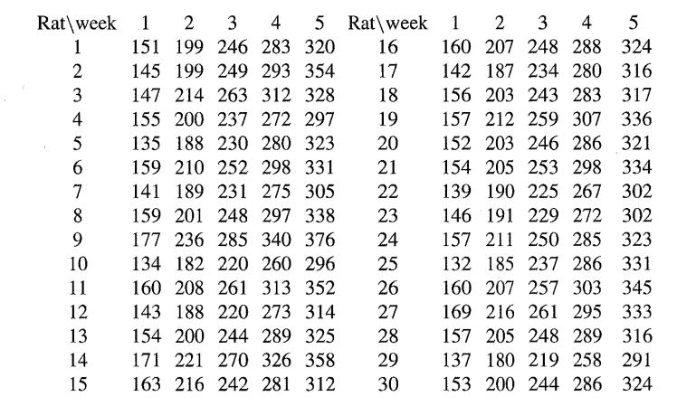
The following data represent the weights of r = 30 young rats measured week! y for n

Question:

The following data represent the weights of r = 30 young rats measured week! y for n = 5 weeks as quoted by Gelfand et al. (1990), Tanner (1996, Table 1.3 and Section 6.2.1), Carlin and Louis (2000, Example 5.6):

$Rat\week 12 1 2 597 A WN 3 4 6 17 3 4 5 151 199 246 283 320 145 199 249 293 354 147 214 263 312 328 155 200$

The weight of the ith rat in week j is denoted X_ij and we suppose that weight growth is linear, that is,

but that the slope and intercept vary from rat to rat. We further suppose that a; and β_i have a bivariate normal distribution, so that a_i

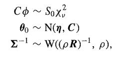
and thus we have a random effects model. At the third stage, we suppose that

Co~ Sox 00 ~ N(n, C) -~W((PR)-, p),

where we have used the notation W(Ω, v) for the Wishart distribution for a random k x k symmetric positive definite matrix V, which has density

p(V | v, ) x | V | (v-k-1)/2 |52|1/2 exp[-Trace(-V)].

Methods of sampling from this distribution are described in Odell and Feiveson (1966), Kennedy and Gentle (1990, Section 6.5.10) and Gelfand et al. (1990). [This example was omitted from the main text because we have avoided use of the Wishart distribution elsewhere in the book. A slightly simpler model in which ∑ is assumed to be diagonal is to be found as the example 'Rats' distributed with WinBUGS.

Explain in detail how you would use the Gibbs sampler to estimate the posterior distributions of a₀ and β₀, and if possible carry out this procedure.

Table 1.3 and Section 6.2.1

1 2 2 Egg no. (i): Length (xi): 22.5 20.1 Breadth (y): 17.0 14.9 16.0 3 4 23.3 22.9 17.4 5 6 6 7 8 9 23.1