New Semester
Started
Get
50% OFF
Study Help!
--h --m --s
Claim Now
Question Answers
Textbooks
Find textbooks, questions and answers
Oops, something went wrong!
Change your search query and then try again
S
Books
FREE
Study Help
Expert Questions
Accounting
General Management
Mathematics
Finance
Organizational Behaviour
Law
Physics
Operating System
Management Leadership
Sociology
Programming
Marketing
Database
Computer Network
Economics
Textbooks Solutions
Accounting
Managerial Accounting
Management Leadership
Cost Accounting
Statistics
Business Law
Corporate Finance
Finance
Economics
Auditing
Tutors
Online Tutors
Find a Tutor
Hire a Tutor
Become a Tutor
AI Tutor
AI Study Planner
NEW
Sell Books
Search
Search
Sign In
Register
study help
business
econometrics
Econometrics 1st Edition Bruce Hansen - Solutions
Consider the just-identified model Y Æ X0 1¯1 Å X0 2¯2 Åe with E[Ze] Æ 0 where X Æ (X0 1X0 2)0 2 Rk and Z 2 Rk . We want to test H0 : ¯1 Æ 0. Three econometricians are called for advice.• Econometrician 1 proposes testing H0 by aWald statistic.• Econometrician 2 suggests testing H0 by
Take the linear equation Y Æ X0¯Åe and consider the following estimators of ¯.1. b¯ : 2SLS using the instruments Z1.2. e¯ : 2SLS using the instruments Z2.3. ¯ : GMMusing the instruments Z Æ (Z1,Z2) and the weight matrix W = (ZZ) 0 0 (Z2Z2) (1-1) for 1 (0,1). Find an expression for which
Consider the model Y Æ X0¯Åe given E[Ze] Æ 0 and R0¯ Æ 0. The dimensions are X 2 Rk and Z 2 R` with ` È k. The matrix R is k £q, 1 · q Ç k. Derive an efficient GMMestimator for ¯.
You want to estimate ¹ Æ E[Y ] under the assumption that E[X] Æ 0, where Y and X are scalar and observed from a random sample. Find an efficient GMMestimator for ¹.
The observations are i.i.d., (Yi ,Xi ,Qi : i Æ 1, ...,n), where X is k £1 and Q is m£1. The model is Y Æ X0¯Åe with E[Xe] Æ 0 and E[Qe] Æ 0. Find the efficient GMMestimator for ¯.
The model is Y Æ Z¯Å X°Åe with E[e j Z] Æ 0, X 2 R and Z 2 R. X is potentially endogenous and Z is exogenous. Someone suggests estimating (¯,°) by GMM using the pair (Z,Z2) as instruments. Is this feasible? Under what conditions is this a valid estimator?
The observed data is {Yi ,Xi ,Zi } 2 R£Rk £R`, k È 1 and ` È k È 1, i Æ 1, ...,n. The model is Y Æ X0¯Åe with E[Ze] Æ 0.(a) Given a weightmatrixW È 0 write down the GMMestimator b¯ for ¯.(b) Suppose the model is misspecified. Specifically, assume that for some ± 6Æ 0, e Æ ±n¡1/2
Consider the model Y Æ X0¯Åe with E[Ze] Æ 0 and R0¯ Æ 0 (13.31)with Y 2 R, X 2 Rk , Z 2 R`, ` È k. The matrix R is k £ q with 1 · q Ç k. You have a random sample(Yi ,Xi ,Zi : i Æ 1, ...,n).For simplicity, assume the efficient weight matrixW Æ¡E£Z Z0e2¤¢¡1 is known.(a) Write out the
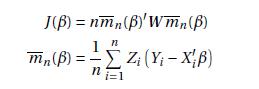
Take the model Y Æ X0¯Åe with E[Ze] Æ 0, Y 2 R, X 2 Rk , Z 2 R`, ` ¸ k. Consider the statisticfor some weight matrixW È 0.(a) Take the hypothesis H0 : ¯ Æ ¯0. Derive the asymptotic distribution of J (¯0) under H0 as n!1.(b) What choice for W yields a known asymptotic distribution in part
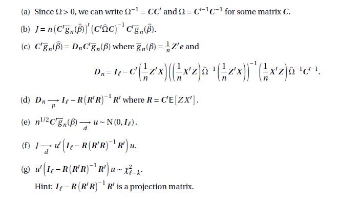
Take the linear model Y Æ X0¯Åe with E[Ze] Æ 0. Consider the GMM estimator b¯ of ¯.Let J Æ n g n( b¯)0b¡1g n( b¯) denote the test of overidentifying restrictions. Show that J ¡!dÂ2`¡k as n !1 by demonstrating each of the following. (a) Since > 0, we can write 2-1 = CC' and Q = CC-1
In the linear model Y Æ X0¯Åe with E[Xe] Æ 0 the GMMcriterion function for ¯ is J (¯) Æ1 n¡Y ¡X ¯¢0 Xb¡1X 0 ¡Y ¡X ¯¢(13.29)where bÆ n¡1PniÆ1 Xi X0 i be2 i , bei Æ Yi ¡ X0 ib¯ are the OLS residuals, and b¯ Æ¡X 0X¢¡1 X 0Y is least squares.The GMMestimator of ¯ subject
derive the efficient GMM estimator using the instrument Z Æ (X X2)0. Does this differ from 2SLS and/or OLS?
As a continuation of
The equation of interest is Y Æm(X,¯)Åe with E[Ze] Æ 0 wherem(x,¯) is a known function,¯ is k £1 and Z is `£1. Show how to construct an efficient GMMestimator for ¯.
Prove Theorem13.10.
Prove Theorem13.9.
Showthat the constrainedGMMestimator (13.16)with the efficientweight matrix is (13.19).
Derive the constrained GMMestimator (13.16).
Prove Theorem13.8.
In the linear model estimated by GMMwith general weight matrixW the asymptotic variance of b¯gmm is V Æ¡Q0WQ¢¡1Q0WWQ¡Q0WQ¢¡1 .(a) Let V 0 be this matrix whenW Æ¡1. Show that V 0 Æ¡Q0¡1Q¢¡1 .(b) Wewant to showthat for anyW, V ¡V 0 is positive semi-definite (for then V 0 is the
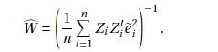
Take the model Y Æ X0¯Åe with E[Ze] Æ 0. Let eei Æ Yi ¡ X0 ie¯ where e¯ is consistent for ¯(e.g. a GMMestimator with some weight matrix). An estimator of the optimal GMMweight matrix isShow that cW ¡!p ¡1 where Æ E £Z Z0e2¤. W = n i=1
Take the model Y Æ X0¯Åe with E[e j Z] Æ 0. Let b¯gmm be the GMM estimator using the weight matrixWn Æ¡Z0Z¢¡1 . Under the assumption E£e2 j Z¤Æ ¾2 show that pn¡ b¯¡¯¢¡!d N³0,¾2 ¡Q0M¡1Q¢¡1´where Q Æ E£Z X0¤and M Æ E£Z Z0¤.
Take themodel Y Æ X0¯Åe E[Xe] Æ 0 e2 Æ Z0°Å´E£Z´¤Æ 0.Find the method of moments estimators¡ b¯, b°¢for¡¯,°¢.
you extended the work reported in Angrist and Krueger (1991) by estimating wage equations for the subsample of Black men. Re-estimate equation (12.92) for this group using as instruments only the three quarter-of-birth dummy variables. Calculate the standard error for the return to education by
In
You will extend Angrist and Krueger (1991) using the data file AK1991 on the textbook website.. Their Table VIII reports estimates of an analog of (12.90) for the subsample of 26,913 Black men. Use this sub-sample for the following analysis.(a) Estimate an equation which is identical in form to
you extended the work reported in Card (1995). Now, estimate the IV equation corresponding to the IV(a) column of Table 12.1 which is the baseline specification considered in Card. Use the bootstrap to calculate a BC percentile confidence interval. In this example should we also report the
In
You will replicate and extend the work reported in the chapter relating to Card (1995).The data is from the author’s website and is posted as Card1995. The model we focus on is labeled 2SLS(a) in Table 12.1 which uses public and private as instruments for edu. The variables you will need for this
you extended the work reported in Acemoglu, Johnson, and Robinson(2001). Consider the 2SLS regression (12.88). Compute the standard errors both by the asymptotic formula and by the bootstrap using a large number (10,000) of bootstrap replications. Re-calculate the bootstrap standard errors. Comment
In
You will replicate and extend the work reported in Acemoglu, Johnson, and Robinson(2001). The authors provided an expanded set of controls when they published their 2012 extension and posted the data on the AER website. This dataset is AJR2001 on the textbook website.(a) Estimate the OLS regression
In the linear model Y Æ X¯Åe with X 2 R suppose ¾2(x) Æ E£e2 j X Æ x¤is known. Show that the GLS estimator of ¯ can be written as an instrumental variables estimator using some instrument Z. (Find an expression for Z.)
The model is Y Æ X0¯Åe with E[Ze] Æ 0. An economist wants to obtain the 2SLS estimates and standard errors for ¯. He uses the following steps• Regresses X on Z, obtains the predicted values bX.• Regresses Y on bX, obtains the coefficient estimate b¯ and standard error s( b¯) from this
You want to use household data to estimate ¯ in the model Y Æ X¯Åe with X scalar and endogenous, using as an instrument the state of residence.(a) What are the assumptions needed to justify this choice of instrument?(b) Is the model just identified or overidentified?
You have two independent i.i.d. samples (Y1i ,X1i ,Z1i : i Æ 1, ...,n) and (Y2i ,X2i ,Z2i : i Æ1, ...,n). The dependent variables Y1 and Y2 are real-valued. The regressors X1 and X2 and instruments Z1 and Z2 are k-vectors. The model is standard just-identified linear instrumental variables Y1 Æ
Take the model Y Æ X0¯ Å e with E[Ze] Æ 0 and consider the two-stage least squares estimator. The first-stage estimate is least squares of X on Z with least squares fitted values bX. The second-stage is least squares of Y on bX with coefficient estimator b¯ and least squares residuals bei ÆYi
Take a linear equation with endogeneity and a just-identified linear reduced form Y ÆX¯Åe with X Æ °Z Åu2 where both X and Z are scalar 1£1. Assume that E[Ze] Æ 0 and E[Zu2] Æ 0.(a) Derive the reduced formequation Y Æ Z¸Åu1. Show that ¯ Æ ¸/° if ° 6Æ 0, and that E[Zu] Æ 0.(b)
Take the linear instrumental variables equation Y1 Æ Z¯1 Å Y2¯2 Å e with E[e j Z] Æ 0 where both X and Z are scalar 1£1.(a) Can the coefficients (¯1,¯2) be estimated by 2SLS using Z as an instrument for Y2?Why or why not?(b) Can the coefficients (¯1,¯2) be estimated by 2SLS using Z and
Take the linear instrumental variables equation Y1 Æ Z0 1¯1ÅY 0 2¯2Åe with E[Ze] Æ 0 where Z1 is k1 £1, Y2 is k2 £1, and Z is `£1, with ` ¸ k Æ k1 Åk2. The sample size is n. Assume that QZ Z ÆE£Z Z0¤È 0 and QZ X Æ E£Z X0¤has full rank k.Suppose that only (Y1,Z1,Z2) are available
Consider the structural equation Y1 Æ Z0 1¯1 ÅY 0 2¯2 Åe with E[Ze] Æ 0 where Y2 is k2 £1 and treated as endogenous. The variables Z Æ (Z1,Z2) are treated as exogenous where Z2 is `2 £1 and`2 ¸ k2. You are interested in testing the hypothesis H0 : ¯2 Æ 0.Consider the reduced
Consider the structural equation and reduced form Y Æ ¯X2 Åe X Æ °Z Åu E[Ze] Æ 0 E[Zu] Æ 0 with X2 treated as endogenous so that E£X2e¤6Æ 0. For simplicity assume no intercepts. Y , Z, and X are scalar. Assume ° 6Æ 0. Consider the following estimator. First, estimate ° by OLS of X on
Consider the structural equation Y Æ ¯0 ů1X ů2X2 Åe (12.93)with X 2 R treated as endogenous so that E[Xe] 6Æ 0. We have an instrument Z 2 R which satisfies E[e j Z] Æ 0 so in particular E[e] Æ 0 , E[Ze] Æ 0 and E£Z2e¤Æ 0.(a) Should X2 be treated as endogenous or exogenous?(b)
Consider the model Y Æ X0¯Åe X Æ ¡0Z Åu E[Ze] Æ 0 E£Zu0¤Æ 0 with Y scalar and X and Z each a k vector. You have a random sample (Yi ,Xi ,Zi : i Æ 1, ...,n). Take the control function equation e Æ u0°Åº with E[uº] Æ 0 and assume for simplicity that u is observed.Inserting into the
Consider the model Y Æ X0¯Åe with E[e j Z] Æ 0 with Y scalar and X and Z each a k vector. You have a randomsample (Yi ,Xi ,Zi : i Æ 1, ...,n).(a) Assume that X is exogenous in the sense that E[e j Z,X] Æ 0. Is the IV estimator b¯iv unbiased?(b) Continuing to assume that X is exogenous, find
Suppose that price and quantity are determined by the intersection of the linear demand and supply curves Demand : Q Æ a0 Åa1P Åa2Y Åe1 Supply : Q Æ b0 Åb1P Åb2W Åe2 where income (Y ) and wage (W) are determined outside the market. In this model are the parameters identified?
Take the linear model Y Æ X0¯Åe with E[e j X] Æ 0 where X and ¯ are 1£1.(a) Show that E[Xe] Æ 0 and E£X2e¤Æ 0. Is Z Æ (X X2)0 a valid instrument for estimation of ¯?(b) Define the 2SLS estimator of ¯ using Z as an instrument for X. How does this differ fromOLS?
For Theorem 12.3 establish that bV ¯ ¡!p V ¯.
In the structural model Y Æ X0¯Åe with X Æ ¡0Z Åu and ¡ `£k, ` ¸ k, we claim that a necessary condition for ¯ to be identified (can be recovered from the reduced form) is rank(¡) Æ k.Explain why this is true. That is, show that if rank(¡) Ç k then ¯ is not identified.
The reduced formbetween the regressors X and instruments Z takes the form X Æ ¡0Z Åu where X is k£1, Z is `£1, and ¡ is `£k. The parameter ¡ is defined by the population moment condition E£Zu0¤Æ 0. Show that the method of moments estimator for ¡ isb¡Æ¡Z0Z¢¡1 ¡Z0X¢.
Take the linear model Y Æ X0¯Åe. Let the OLS estimator for ¯ be b¯ with OLS residual bei .Let the IV estimator for ¯ using some instrument Z be e¯ with IV residual eei Æ Yi ¡ X0 ie¯. If X is indeed endogenous, will IV “fit” better than OLS in the sense that PniÆ1 ee2 iÇPniÆ1 be2 i
Take the linear model Y Æ X0¯ Å e with E[e j X] Æ 0. Suppose ¾2(x) Æ E£e2 j X Æ x¤is known. Show that the GLS estimator of ¯ can be written as an IV estimator using some instrument Z. (Find an expression for Z.)
Consider the single equationmodel Y Æ Z¯Åe where Y and Z are both real-valued (1£1).Let b¯ denote the IV estimator of ¯ using as an instrument a dummy variable D (takes only the values 0 and 1). Find a simple expression for the IV estimator in this context.
The observations are i.i.d., (Y1i ,Y2i ,Xi : i Æ 1, ...,n). The dependent variables Y1 and Y2 are real-valued. The regressor X is a k-vector. The model is the two-equation system(a) What are the appropriate estimators b¯1 and b¯2 for ¯1 and ¯2?(b) Find the joint asymptotic distribution of b¯1
Take themodelwhere Y is scalar, X is a k vector and Z is an ` vector. ¯ and ¼ are k £1 and ¡ is `£k. The sample is (Yi ,Xi ,Zi : i Æ 1, ...,n) with ¼i unobserved.Consider the estimator b¯ for ¯ by OLS of Y onb¼Æb¡0Z whereb¡is the OLS coefficient from the multivariate regression of X on
Prove Theorem11.6.
Prove Theorem11.5.Hint: First, show that it is sufficient to show thatSecond, rewrite this equation using the transformations U Æ §1/2X and V Æ §1/2X, and then apply the matrix Cauchy-Schwarz inequality (B.33). EXX (EXEXX EXX.
Prove Theorem11.4.
Show that (11.17) follows from the steps described.
Show that (11.16) follows from the steps described.
Prove Theorem11.3.
Prove Theorem11.2.
Show (11.14) when the regressors are common across equations Xj Æ X and the errors are conditionally homoskedastic (11.8).
Show (11.13) when the regressors are common across equations Xj Æ X.
Prove Theorem11.1.
Show (11.12) when the regressors are common across equations Xj Æ X and the errors are conditionally homoskedastic (11.8).
Show (11.11) when the regressors are common across equations Xj Æ X.
Show (11.10) when the errors are conditionally homoskedastic (11.8).
you extended the work from Duflo, Dupas, and Kremer (2011). Repeat that regression, nowcalculating the standard error by cluster bootstrap. Report a BCa confidence interval for each coefficient.
In
you estimated a wage regression with the cps09mar dataset and the subsample of whiteMale Hispanics. Further restrict the sample to those never-married and live in theMidwest region. (This sample has 99 observations.) As in subquestion (b) let µ be the ratio of the return to one year of education
In
you estimated the Mankiw, Romer, and Weil (1992) unrestricted regression.Let µ be the sum of the second, third, and fourth coefficients.(a) Estimate the regression by unrestricted least squares and report standard errors calculated by asymptotic, jackknife and the bootstrap.(b) Estimate µ and
In
you estimated a cost function for 145 electric companies and tested the restriction µ Æ ¯3 ů4 ů5 Æ 1.(a) Estimate the regression by unrestricted least squares and report standard errors calculated by asymptotic, jackknife and the bootstrap.(b) Estimate µ Æ ¯3 ů4 ů5 and report
In
Themodel is Y Æ X0¯Åe with E[Xe] 6Æ 0. We know that in this case, the least squares estimator may be biased for the parameter ¯.We also know that the nonparametric BC percentile interval is(generally) a good method for confidence interval construction in the presence of bias. Explain whether
The RESET specification test for nonlinearity in a random sample (due to Ramsey (1969))is the following. The null hypothesis is a linear regression Y Æ X0¯Åe with E[e j X] Æ 0. The parameter ¯ is estimated by OLS yielding predicted values b Yi . Then a second-stage least squares regression is
The model is i.i.d. data, i Æ 1, ...,n, Y Æ X0¯Åe and E[e j X] Æ 0. Does the presence of conditional heteroskedasticity invalidate the application of the nonparametric bootstrap? Explain.
Take the model Y Æ X1¯1 Å X2¯2 Åe with i.i.d observations, E[Xe] Æ 0 and scalar X1 and X2. Describe how you would construct the percentile-t bootstrap confidence interval for µ Æ ¯1/¯2.
Take the model Y Æ X1¯1 Å X2¯2 Åe with E[Xe] Æ 0 and scalar X1 and X2. The parameter of interest is µ Æ ¯1¯2. Show how to construct a confidence interval for µ using the following three methods.(a) Asymptotic Theory.(b) Percentile Bootstrap.(c) Percentile-t Bootstrap.Your answer should
Suppose a Ph.D. student has a sample (Yi ,Xi ,Zi : i Æ 1, ...,n) and estimates by OLS the equation Y Æ Z®Å X0¯Åe where ® is the coefficient of interest. She is interested in testing H0 : ® Æ 0 against H1 : ® 6Æ 0. She obtains b®Æ 2.0 with standard error s(b®) Æ 1.0 so the value of
The model is Y Æ X0 1¯1ÅX0 2¯2Åe with E[Xe] Æ 0, and both X1 and X2 k£1. Describe how to test H0 : ¯1 Æ ¯2 against H1 : ¯1 6Æ ¯2 using the nonparametric bootstrap.
The model is Y Æ X0 1¯1 Å X0 2¯2 Åe with E[Xe] Æ 0 and X2 scalar. Describe how to test H0 : ¯2 Æ 0 against H1 : ¯2 6Æ 0 using the nonparametric bootstrap.
Take themodel Y Æ X0¯Åe with E[Xe] Æ 0. Describe the bootstrap percentile confidence interval for ¾2 Æ E£e2¤.
The observed data is {Yi ,Xi } 2 R£Rk , k È 1, i Æ 1, ...,n. Take the model Y Æ X0¯Åe with E[Xe] Æ 0.(a) Write down an estimator for ¹3 Æ E£e3¤.(b) Explain how to use the percentile method to construct a 90% confidence interval for ¹3 in this specific model.
Consider the model Y Æ X0¯Åe with E[e j X] Æ 0, Y scalar, and X a k vector. You have a random sample (Yi ,Xi : i Æ 1, ...,n). You are interested in estimating the regression function m(x) ÆE[Y j X Æ x] at a fixed vector x and constructing a 95% confidence interval.(a) Write down the standard
Take the normal regression model Y Æ X0¯Åe with e j X » N(0,¾2) where we know the MLE equals the least squares estimators b¯ and b¾2.(a) Describe the parametric regression bootstrap for this model. Show that the conditional distribution of the bootstrap observations is Y ¤i j Fn »N¡X0
Suppose that in an application, bµ Æ 1.2 and s(bµ) Æ 0.2. Using the nonparametric bootstrap, 1000 samples are generated from the bootstrap distribution, and bµ¤ is calculated on each sample.The bµ¤ are sorted, and the 0.025th and 0.975th quantiles of the bµ¤ are .75 and 1.3,
You want to test H0 : µ Æ 0 against H1 : µ È 0. The test for H0 is to reject if Tn Æ bµ/s(bµ) È c where c is picked so that Type I error is ®. You do this as follows. Using the nonparametric bootstrap, you generate bootstrap samples, calculate the estimates bµ¤ on these samples and then
Show that if the percentile-t interval for ¯ is [L,U] then the percentile-t interval for aÅc¯is [a ÅbL,a ÅbU].
Take p¤ as defined in (10.22) for the BC percentile interval. Show that it is invariant to replacing µ with g (µ) for any strictly monotonically increasing transformation g (µ). Does this extend to z¤0 as defined in (10.23)?
Consider the following bootstrap procedure for a regression of Y on X. Let b¯ denote the OLS estimator and bei Æ Yi ¡X0 ib¯ the OLS residuals.(a) Draw a random vector (X¤,e¤) from the pair {(Xi , bei ) : i Æ 1, ...,n} . That is, draw a random integer i 0 from [1,2, ...,n], and set X¤ Æ Xi
Let Yi be i.i.d., ¹ Æ E[Y ] È 0, and µ Æ ¹¡1. Let b¹ Æ Y n be the samplemean and bµ Æ b¹¡1.(a) Is bµ unbiased for µ?(b) If bµ is biased, can you determine the direction of the bias E£bµ¡µ¤(up or down)?(c) Is the percentile interval appropriate in this context for confidence
Prove Theorem10.8.
Prove Theorem10.7.
Prove Theorem10.6.
Consider the following bootstrap procedure. Using the nonparametric bootstrap, generate bootstrap samples, calculate the estimate bµ¤ on these samples and then calculate T ¤Æ (bµ¤¡ bµ)/s(bµ), where s(bµ) is the standard error in the original data. Let q¤®/2 and q¤1¡®/2 denote the
Show that if the percentile interval for ¯ is [L,U] then the percentile interval for a Åc¯ is[a ÅcL,a ÅcU].
Showthat if the bootstrap estimator of variance of b¯ is bV boot b¯ , then the bootstrap estimator of variance of bµ Æ a ÅC b¯ is bV boot bµÆC bV boot b¯ C0.
Showing 1400 - 1500
of 4105
First
8
9
10
11
12
13
14
15
16
17
18
19
20
21
22
Last
Step by Step Answers