Employment in different areas, part 3.

In Exercise 19, we raised questions about District of Columbia’s mean annual wage. After removing them together with two lowest residual points from Alaska, the resulting regression looks like this.

Dependent variable is: the mean annual wage ($)

R-squared = 0.1302, Adjusted R-squared: 0.0852 SE = 24569.9144 with 62 observations Variable Coefficient SE(Coeff) t-ratio P-value Intercept 62058.1449 5647.9884 10.9877 0.0000 Total Employment -0.2747 0.0971 -2.8281 0.0064 Jobs 325.6577 154.3140 2.1104 0.0392 Area -6456.6389 7875.2789 -0.8199 0.4157 A plot of the residuals against the predicted values for this regression looks like this. It has been colored according to the different area.

a) What does this plot say about how the regression model deals with these three different areas?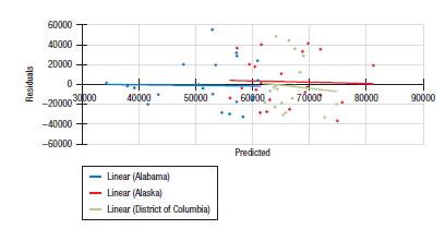

We constructed another variable consisting of the indicator variable Area multiplied by Total employment and Jobs. Here is the resulting regression.
Dependent variable is: the mean annual wage ($)
R-squared = 0.1533, Adjusted R-squared: 0.0939 SE = 24453.2465 with 62 observations Variable Coefficient SE(Coeff) t-ratio P-value Intercept 59911.4137 5878.9144 10.1909 0.0000 Total Employment -0.3316 0.1069 -3.1020 0.0030 Jobs 455.2731 185.4530 2.4549 0.0172 Area -740.4488 9080.1087 -0.0815 0.9353 Area*Total Emp*Jobs -0.0120 0.0096 -1.2469 0.2175

b) Interpret the coefficient of Area*TotalEmp*Jobs in this regression model.

c) Is this a better regression model than the ones in Exercises 17 and 19?

Transcribed Image Text:

Residuals 60000 40000 20000 -20000 -40000 -60000 0 30000 40000 50000 60000 -70000 80000 90000 -Linear (Alabama) Linear (Alaska) Linear (District of Columbia) Predicted