Consider the Barberis et al. [150] model described by equations (9.5)(9.9). In this exercise, following the Appendix of Barberis et al. [150], we provide the proof of Proposition 9.5. Denote by \((w, c):=\left(\left(w_{t}, c_{t}\right)\right)_{t \in \mathbb{N}}\) a self-financing trading-consumption strategy, where the investment strategy \(w_{t+1}\) is parameterized in terms of the amount of wealth invested in the single risky asset between date \(t\) and date \(t+1\). In the context of the present exercise, we assume that a tradingconsumption strategy \((w, c)\) is admissible if \(w_{t}\) is bounded, for all \(t \in \mathbb{N}\). Similarly as in relations (6.4) and (6.19), it is easy to see that a trading-consumption strategy \((\theta, c)\) satisfies the following self-financing condition:

\[W_{t+1}=\left(W_{t}-c_{t}\right) r_{f}+w_{t+1}\left(r_{t+1}-r_{f}\right)+y_{t+1}, \quad \text { for all } t \in \mathbb{N},\]

where \(\left(W_{t}\right)_{t \in \mathbb{N}}\) denotes the self-financing wealth process associated with the strategy \((w, c)\) and \(\left(y_{t}\right)_{t \in \mathbb{N}}\) is the exogenous income stream.

(i) Let \(\left(w^{*}, c^{*}\right)=\left(\left(w_{t}^{*}, c_{t}^{*}\right)\right)_{t \in \mathbb{N}}\) be a trading-consumption strategy satisfying the above self-financing condition. Let \((w, c)=\left(\left(w_{t}, c_{t}\right)\right)_{t \in \mathbb{N}}\) be an alternative selffinancing strategy and define the strategy

\[\left(w^{*}+\alpha w, c^{*}+\alpha c\right)=\left(\left(w_{t}^{*}+\alpha w_{t}, c_{t}^{*}+\alpha c_{t}\right)\right)_{t \in \mathbb{N}},\]

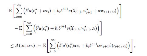
for \(\alpha \in \mathbb{R}_{+}\). Show that, according to the preference functional (9.7), the difference in the expected utilities associated to

and \(\left(c^{*}, w^{*}\right)\)

satisfies

 

where the function \(\hat{v}\) is defined as in the statement of Proposition 9.5.
(ii) Suppose that, for all \(t \in \mathbb{N}\), it holds that \[\begin{gather*}
u^{\prime}\left(c_{t}^{*}\right)=r_{f} \delta \mathbb{E}\left[u^{\prime}\left(c_{t+1}^{*}\right) \mid \mathscr{F}_{t}\right] \tag{9.81}\\u^{\prime}\left(c_{t}^{*}\right)=\delta \mathbb{E}\left[u^{\prime}\left(c_{t+1}^{*}\right) r_{t+1} \mid \mathscr{F}_{t}\right]+\delta b_{t} \mathbb{E}\left[\hat{v}\left(r_{t+1}, z_{t}\right) \mid \mathscr{F}_{t}\right]\tag{9.82}\end{gather*}\]
with \(u(x)=x^{1-\gamma} /(1-\gamma)\) and where the function \(\hat{v}(\cdot)\) is defined as in Proposition 9.5 and the process \(\left(b_{t}\right)_{t \in \mathbb{N}}\) is specified by \(b_{t}=b_{0} \bar{c}_{t}^{-\gamma}\), for all \(t \in \mathbb{N}\). Show that, for all \(t \in \mathbb{N}\), it holds that \(\mathbb{E}\left[u^{\prime}\left(c_{t}^{*}\right) \alpha c_{t}+\alpha w_{t+1} \delta b_{t} \hat{v}\left(r_{t+1}, z_{t}\right) \mid \mathscr{F}_{t}\right]=u^{\prime}\left(c_{t}^{*}\right) \alpha W_{t}-\delta \mathbb{E}\left[u^{\prime}\left(c_{t+1}^{*}\right) \alpha W_{t+1} \mid \mathscr{F}_{t}\right]\), where \(\left(W_{t}\right)_{t \in \mathbb{N}}\) is the wealth process associated to the self-financing strategy \((w, c)\).
(iii) Deduce that

 

As explained in Barberis et al. [150, Appendix], the right-hand side of the last equality vanishes if \(W_{0}=0\) and the following condition holds:
\[\log \delta-\gamma g_{c}+g_{d}+\frac{\gamma^{2} \sigma_{c}^{2}-2 \gamma ho \sigma_{c} \sigma_{d}+\sigma_{d}^{2}}{2}

This shows that the Euler conditions (9.81)-(9.82) are necessary and sufficient for the optimality of the strategy \(\left(\left(\theta_{t}^{*}, c_{t}^{*}\right)\right)_{t \in \mathbb{N}}\).
(iv) Show that the risk free return \(r_{f}\) given in (9.10) satisfies the Euler condition (9.81) when the consumption process \(\left(c_{t}^{*}\right)_{t \in \mathbb{N}}\) is given by the aggregate per capita consumption process \(\left(\bar{c}_{t}\right)_{t \in \mathbb{N}}\).

(v) Suppose that the equilibrium price-dividend ratio of the risky asset satisfies \[\frac{p_{t}^{*}}{d_{t}}=f\left(z_{t}\right), \quad \text { for all } t \in \mathbb{N}\]
for a suitable function \(f(\cdot)\). Show that

 

Deduce that condition (9.11) of Proposition 9.5 implies that the Euler optimality condition (9.82) holds.
(vi) Deduce that the strategy of consuming \(c_{t}^{*}=\bar{c}_{t}=d_{t}+y_{t}\), for all \(t \in \mathbb{N}\), and holding the market supply of the risky asset satisfies the Euler conditions (9.81)-(9.82) and the claim of Proposition 9.5 follows.

Transcribed Image Text:

(c* +ac, w*+aw)