Question:
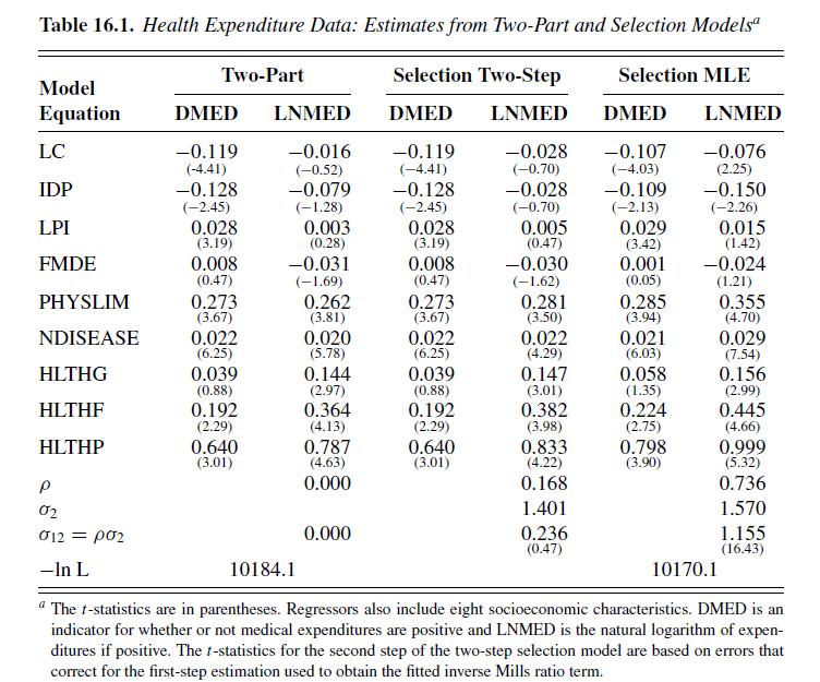
Use the health expenditure data of Section 16.6. The model is a probit regression of DMED, an indicator variable for positive health expenditures, against the 17 regressors listed in the second paragraph of Section 16.6. You should obtain the estimates given in the first column of Table 16.1.
(a) Test the joint statistical significance of the self-rated health indicators HLTHG, HLTHF, and HLTHP at level 0.05 using a Hausman test. [This may require some additional coding, depending on the package used.]
(b) Is the Hausman test the best test to use here?
(c) Does an information matrix test at level 0.05 support the restrictions of this model? [This will require some additional coding.]
(d) Discriminate between a model that drops HLTHG, HLTHF, and HLTHP and a model that drops LC, IDP, and LPI on the basis of \(R_{\mathrm{RES}}^{2}, R_{\mathrm{EXP}}^{2}, R_{\mathrm{COR}}^{2}\), and \(R_{\mathrm{RG}}^{2}\).


Transcribed Image Text:
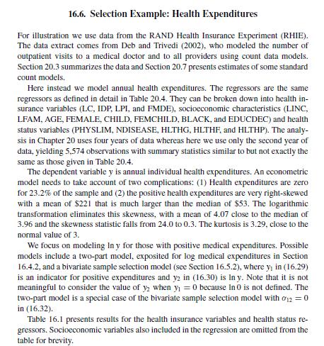
16.6. Selection Example: Health Expenditures For illustration we use data from the RAND Health Insurance Experiment (RHIE). The data extract comes from Deb and Trivedi (2002), who modeled the number of outpatient visits to a medical doctor and to all providers using count data models. Section 20.3 summarizes the data and Section 20.7 presents estimates of some standard count models. Here instead we model annual health expenditures. The regressors are the same regressors as defined in detail in Table 20.4. They can be broken down into health in- surance variables (LC, IDP, LPI, and FMDE), socioeconomic characteristics (LINC, LFAM, AGE, FEMALE, CHILD, FEMCHILD, BLACK, and EDUCDEC) and health status variables (PHYSLIM, NDISEASE, HLTHG, HLTHF, and HLTHP). The analy- sis in Chapter 20 uses four years of data whereas here we use only the second year of data, yielding 5,574 observations with summary statistics similar to but not exactly the same as those given in Table 20.4. The dependent variable y is annual individual health expenditures. An econometric model needs to take account of two complications: (1) Health expenditures are zero for 23.2% of the sample and (2) the positive health expenditures are very right-skewed with a mean of $221 that is much larger than the median of $53. The logarithmic transformation eliminates this skewness, with a mean of 4.07 close to the median of 3.96 and the skewness statistic falls from 24.0 to 0.3. The kurtosis is 3.29, close to the normal value of 3. We focus on modeling In y for those with positive medical expenditures. Possible models include a two-part model, exposited for log medical expenditures in Section 16.4.2, and a bivariate sample selection model (see Section 16.5.2), where y; in (16.29) is an indicator for positive expenditures and y2 in (16.30) is In y. Note that it is not meaningful to consider the value of y when y = 0 because In 0 is not defined. The two-part model is a special case of the bivariate sample selection model with 012 = 0 in (16.32). Table 16.1 presents results for the health insurance variables and health status re- gressors. Socioeconomic variables also included in the regression are omitted from the table for brevity.
