Use the health expenditure data of Section 16.6. The model is a probit regression of DMED, an indicator variable for positive health expenditures, against just one regressor for simplicity, NDISEASE, the number of chronic diseases.

(a) Obtain the OLS estimate of the slope parameter.

(b) Obtain the probit estimate of the slope parameter.

(c) Given part (b), obtain the marginal effect of chronic diseases in two ways: averaged over the sample and evaluated at the sample average of NDISEASE.

(d) Obtain the logit estimate of the slope parameter.

(e) Given part (d), obtain the marginal effect of chronic diseases in three ways: averaged over the sample, evaluated at the sample average of NDISEASE, and evaluated at \(\Lambda\left(\mathbf{x}^{\prime} \beta\right)=\bar{y}\).

(f) For the logit model calculate the proportionate change in the odds ratio when NDISEASE changes.

Transcribed Image Text:

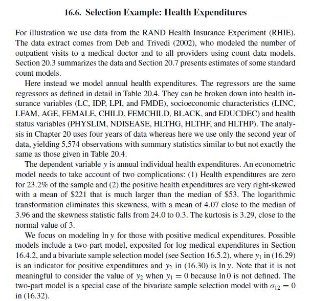
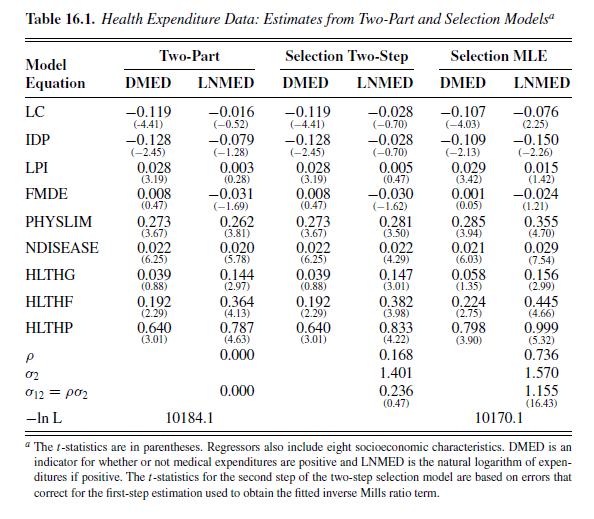
16.6. Selection Example: Health Expenditures For illustration we use data from the RAND Health Insurance Experiment (RHIE). The data extract comes from Deb and Trivedi (2002), who modeled the number of outpatient visits to a medical doctor and to all providers using count data models. Section 20.3 summarizes the data and Section 20.7 presents estimates of some standard count models. Here instead we model annual health expenditures. The regressors are the same regressors as defined in detail in Table 20.4. They can be broken down into health in- surance variables (LC, IDP, LPI, and FMDE), socioeconomic characteristics (LINC, LFAM, AGE, FEMALE, CHILD, FEMCHILD, BLACK, and EDUCDEC) and health status variables (PHYSLIM, NDISEASE, HLTHG, HLTHF, and HLTHP). The analy- sis in Chapter 20 uses four years of data whereas here we use only the second year of data, yielding 5,574 observations with summary statistics similar to but not exactly the same as those given in Table 20.4. The dependent variable y is annual individual health expenditures. An econometric model needs to take account of two complications: (1) Health expenditures are zero for 23.2% of the sample and (2) the positive health expenditures are very right-skewed with a mean of $221 that is much larger than the median of $53. The logarithmic transformation eliminates this skewness, with a mean of 4.07 close to the median of 3.96 and the skewness statistic falls from 24.0 to 0.3. The kurtosis is 3.29, close to the normal value of 3. We focus on modeling In y for those with positive medical expenditures. Possible models include a two-part model, exposited for log medical expenditures in Section 16.4.2, and a bivariate sample selection model (see Section 16.5.2), where y; in (16.29) is an indicator for positive expenditures and y2 in (16.30) is In y. Note that it is not meaningful to consider the value of y2 when y = 0 because In 0 is not defined. The two-part model is a special case of the bivariate sample selection model with 12 = 0 in (16.32).