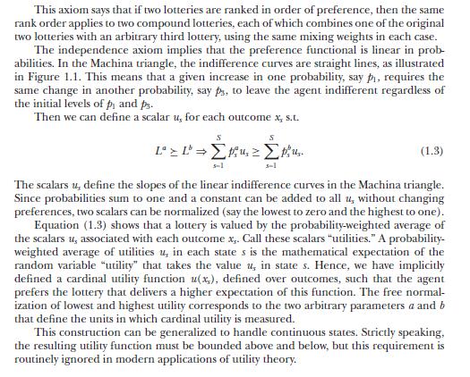
Long-run risk models offer a solution to the main asset pricing puzzles by assuming that there exists a representative agent with Epstein-Zin preferences with moderately high risk aversion and a high elasticity of intertemporal substitution and that aggregate consumption growth is persistent and conditionally heteroskedastic. In this problem we explore the implications of such a setting (preference and endowment specification) for the representative agent's attitudes toward the temporal resolution of uncertainty.

Consider an infinite-horizon endowment economy. The representative agent has Epstein-Zin utility, defined recursively in (6.34) and (6.35). Consumption follows an exogenous process given by

Equation 6.100 and 6.101

Equation 6.34

Equation 6.35

where \(c_{t} \equiv \log C_{t}\), and \(\eta_{t}\) and \(e_{t}\) are standard normal variables, mutually independent and iid over time. \({ }^{11}\)

(a) Explain intuitively why \(\gamma-1 / \psi>0\) implies a preference for early resolution of uncertainty.

(b) Recall the discussion of the risk premium in section 1.2. The timing premium, \(\pi^{*}\), can be defined analogously as the (maximum) fraction of the consumption stream that one would give up at date 0 in order to have all risk resolved at date 1 . That is, the agent is indifferent between consuming the stream \(C=\left\{C_{t}ight\}_{t=0}^{\infty}\) given by (6.100) and (6.101) with risk resolved gradually and consuming the stream \(\left(1-\pi^{*}ight) C=\) \(\left\{\left(1-\pi^{*}ight) C_{t}ight\}_{t=0}^{\infty}\) while learning the realizations of \(C_{1}, C_{2}, C_{3}, \ldots\) with certainty at date 1 .
Let \(U_{0}\) denote the utility at date 0 from consuming \(C\) with risk resolved gradually and let \(U_{0}^{*}\) denote the utility at date 0 from consuming \(C\) with risk resolved at date 1. Show that, for Epstein-Zin preferences, the timing premium can be written as

For the remaining parts assume that \(\psi=1\), a case that admits a closed-form solution.

(c) Guess and verify that \(U_{0}\) is given by

(d) Calculate \(U_{0}^{*}\) by first solving for \(U_{1}^{*}\), the utility from a deterministic consumption stream, as \(\log U_{1}^{*}=c_{0}+\sum_{t=1}^{\infty} \delta^{t-1} \Delta c_{t}\) and then solving for \(U_{0}^{*}\) given the date- 0 conditional distribution of \(U_{1}^{*}\). Show that the timing premium, (6.102), equals

Equation 6.102

Explain why, for \(\gamma>1\), the timing premium is increasing in \(\gamma, \delta, \sigma, \varphi_{e}\), and \(ho_{x}\).

(e) Give a numerical estimate for the timing premium given the following parameter values from Bansal and Yaron (2004): \(\sigma=0.0078, \varphi_{e}=0.044, ho_{x}=0.979, \delta=0.998\), and \(\gamma=7.5\). Repeat with \(\gamma=10\). Assess these estimates through introspection: would you be willing to give such a fraction of your entire consumption stream in order to know your consumption stream with certainty earlier in your life? Note that the question at hand is about consumption risk, not about income or return risk; that is, there is no instrumental value in knowing your consumption in advance.

(f) Finally, we ask whether a high EIS necessarily implies very high timing premia or whether the results of part

(e) are due to the particular combination of preferences and endowment process frequently assumed in the long-run risk literature. Repeat part

(e) under the assumption of an iid consumption growth process, that is, by setting \(ho_{x}=\varphi_{e}=0\). How do these estimates compare to those of part (e)? Explain intuitively why, given the assumed preferences (high \(\gamma\) and \(\gamma>1 / \psi)\), a persistent process for consumption growth is associated with high timing premia.

Data from section 1.2

Transcribed Image Text:

= Met xi + ant1, X4+1 = + , (6.100) (6.101)