Answered step by step
Verified Expert Solution
Question
1 Approved Answer
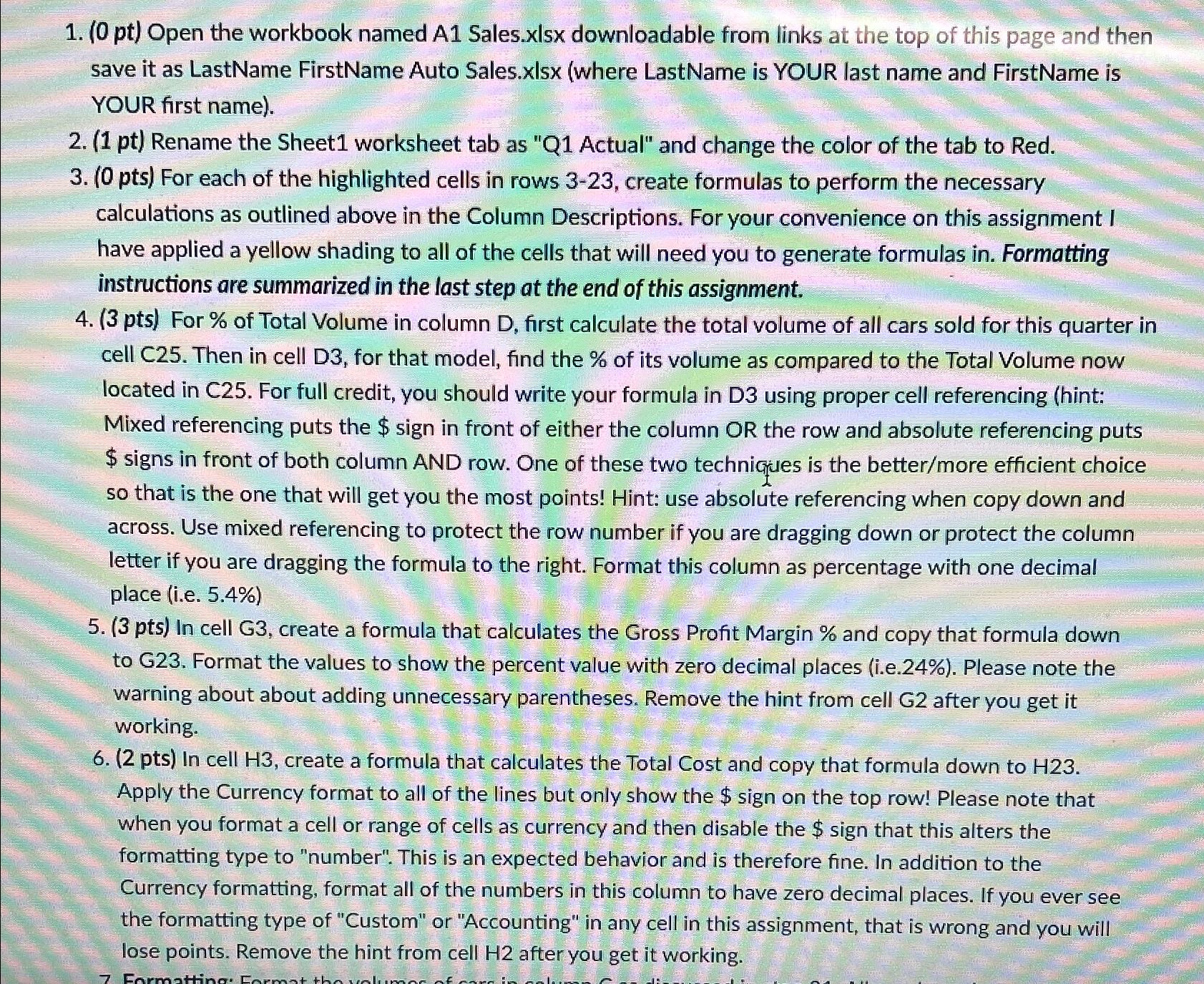
( 0 pt ) Open the workbook named A 1 Sales.xlsx downloadable from links at the top of this page and then save it as
pt Open the workbook named A Sales.xlsx downloadable from links at the top of this page and then save it as LastName FirstName Auto Sales.xlsx where LastName is YOUR last name and FirstName is YOUR first name
pt Rename the Sheet worksheet tab as Q Actual" and change the color of the tab to Red.
pts For each of the highlighted cells in rows create formulas to perform the necessary calculations as outlined above in the Column Descriptions. For your convenience on this assignment I have applied a yellow shading to all of the cells that will need you to generate formulas in Formatting instructions are summarized in the last step at the end of this assignment.
pts For of Total Volume in column D first calculate the total volume of all cars sold for this quarter in cell C Then in cell D for that model, find the of its volume as compared to the Total Volume now located in C For full credit, you should write your formula in D using proper cell referencing hint: Mixed referencing puts the $ sign in front of either the column OR the row and absolute referencing puts $ signs in front of both column AND row. One of these two techniques is the bettermore efficient choice so that is the one that will get you the most points! Hint: use absolute referencing when copy down and across. Use mixed referencing to protect the row number if you are dragging down or protect the column letter if you are dragging the formula to the right. Format this column as percentage with one decimal place ie
pts In cell G create a formula that calculates the Gross Profit Margin and copy that formula down to G Format the values to show the percent value with zero decimal places ie Please note the warning about about adding unnecessary parentheses. Remove the hint from cell G after you get it working.
pts In cell H create a formula that calculates the Total Cost and copy that formula down to Apply the Currency format to all of the lines but only show the $ sign on the top row! Please note that when you format a cell or range of cells as currency and then disable the $ sign that this alters the formatting type to "number". This is an expected behavior and is therefore fine. In addition to the Currency formatting, format all of the numbers in this column to have zero decimal places. If you ever see the formatting type of "Custom" or "Accounting" in any cell in this assignment, that is wrong and you will lose points. Remove the hint from cell after you get it working.

Step by Step Solution
There are 3 Steps involved in it
Step: 1

Get Instant Access to Expert-Tailored Solutions
See step-by-step solutions with expert insights and AI powered tools for academic success
Step: 2

Step: 3

Ace Your Homework with AI
Get the answers you need in no time with our AI-driven, step-by-step assistance
Get Started


