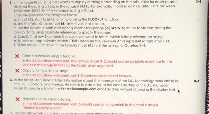
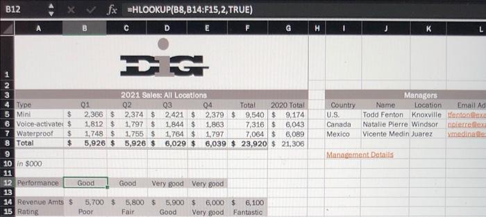
0/4 5. In the range B12:E12. Benicio wants to display a rating depending on the total sales for each quarter. He isted the rating criteria in the range A14:F15. For example, if total sales in Quarter I are between $5900 and $5999, the Performance rating is Good. Enter the performance ratings as follows: a. In cell B12. start to enter a formula using the HLOOKUP function. b. Use the Total Q1 sales (cell B8) as the value to look up. c. Use the Revenue Arts and Rating infomation (range $B$14:$F$15) as the table containing the lookup data, using absolute references to specify the range. d. Specity that row 2 contains the value you want to return, which is the performance rating. e. Specify an approximate match (TRUE) because the Revenue Amts represent ranges of values. f. Fil the range C12:E12 with the formula in cell B12 to enter ratings for Quarters 2-4. X Create a formula using a function. In the Allocations worksheet, the formula in cell B12 should use an absolute reference to the values in the range B14:F15 as the table_array argument. X Copy a formula into a range. In the All Location worksheet cell B12 contains an incorrect formula 6. In the range 13:17. Benicio listed information about the managers of the DIG Technology main offices in the U., Canada, and Mexico. He needs to add a link to the email address of the U.S. manager. In cell L5, create a link to the tenton@example.com email address without changing the display text 0/4 WWWLWNNW x Hyperlink to an email address In the All Locations worksheet, cell LS should contain a hyperlink to the email address Tenton@example.com 7 Rani in no want to move B12 XV fx =HLOOKUP(B8,B14:F15,2, TRUE) F G J K L PG Country U.S. Canada Mexico Managers Name Location Email Ad Todd Fenton Knoxville tentontex Natalie Pierre Windsor noen Vicente Medin Juarez ymedia 2021 Sales: All Locations 4 Type 01 Q2 Q3 04 Total 2020 Total 5 Mini $ 2,366 $ 2,374 $ 2.421 $ 2.379 $ 9,540 $ 9,174 6 Voice-activate: $ 1.812 $ 1,797 $ 1 844 $ 1,863 7,316 $ 6,043 7 Waterproof $ 1,748 $ 1,755 $ 1,764 $ 1,797 7,064 $ 6,089 8 Total $ 5,926 $ 5,926 $ 6,029 $ 6,039 $ 23,920 $ 21,306 9 10 in 8000 11 12 Performance Good Good Very good Very good 13 14 Revenue Amts $ 5,700 $ 5,800 $ 5,900 $ 6,000 $ 6,100 15 Rating Poor Fair Good Very good Fantastic Management Details 0/4 5. In the range B12:E12. Benicio wants to display a rating depending on the total sales for each quarter. He isted the rating criteria in the range A14:F15. For example, if total sales in Quarter I are between $5900 and $5999, the Performance rating is Good. Enter the performance ratings as follows: a. In cell B12. start to enter a formula using the HLOOKUP function. b. Use the Total Q1 sales (cell B8) as the value to look up. c. Use the Revenue Arts and Rating infomation (range $B$14:$F$15) as the table containing the lookup data, using absolute references to specify the range. d. Specity that row 2 contains the value you want to return, which is the performance rating. e. Specify an approximate match (TRUE) because the Revenue Amts represent ranges of values. f. Fil the range C12:E12 with the formula in cell B12 to enter ratings for Quarters 2-4. X Create a formula using a function. In the Allocations worksheet, the formula in cell B12 should use an absolute reference to the values in the range B14:F15 as the table_array argument. X Copy a formula into a range. In the All Location worksheet cell B12 contains an incorrect formula 6. In the range 13:17. Benicio listed information about the managers of the DIG Technology main offices in the U., Canada, and Mexico. He needs to add a link to the email address of the U.S. manager. In cell L5, create a link to the tenton@example.com email address without changing the display text 0/4 WWWLWNNW x Hyperlink to an email address In the All Locations worksheet, cell LS should contain a hyperlink to the email address Tenton@example.com 7 Rani in no want to move B12 XV fx =HLOOKUP(B8,B14:F15,2, TRUE) F G J K L PG Country U.S. Canada Mexico Managers Name Location Email Ad Todd Fenton Knoxville tentontex Natalie Pierre Windsor noen Vicente Medin Juarez ymedia 2021 Sales: All Locations 4 Type 01 Q2 Q3 04 Total 2020 Total 5 Mini $ 2,366 $ 2,374 $ 2.421 $ 2.379 $ 9,540 $ 9,174 6 Voice-activate: $ 1.812 $ 1,797 $ 1 844 $ 1,863 7,316 $ 6,043 7 Waterproof $ 1,748 $ 1,755 $ 1,764 $ 1,797 7,064 $ 6,089 8 Total $ 5,926 $ 5,926 $ 6,029 $ 6,039 $ 23,920 $ 21,306 9 10 in 8000 11 12 Performance Good Good Very good Very good 13 14 Revenue Amts $ 5,700 $ 5,800 $ 5,900 $ 6,000 $ 6,100 15 Rating Poor Fair Good Very good Fantastic Management Details


