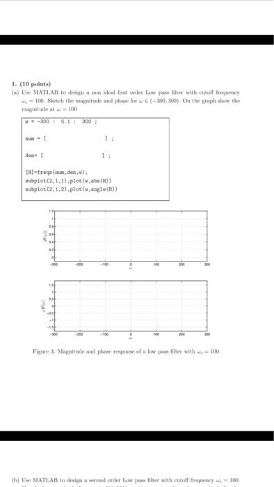
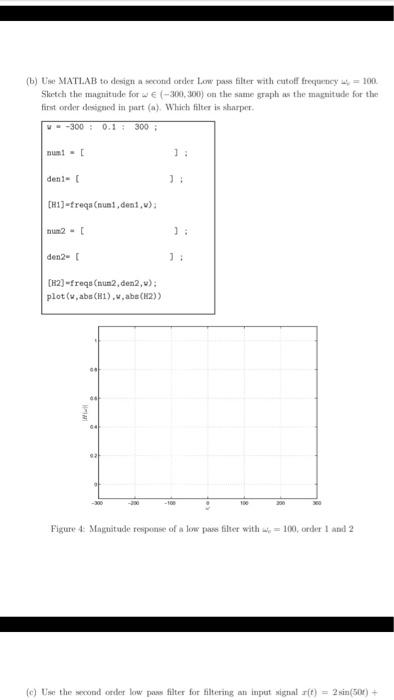
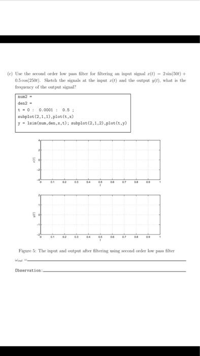
1. (10 points) {m) U MATLAB to desta com ideal first one low peefilter with custoll frequency Wi = 100. Sktch the mapuitude and phone for w (-300, 300). On the graph who magnitude - 100 V-3000.11 300 1 det [H]-frequum,den,w). subplot(2,1,1).plot(.abs()) subplot(2,1,2).plot(.angle(H)) 13 al 94 03 00 200 - -18 18 Figure 3: Magnitude and phase response of a low pa filter with : 100 (b) Use MATLAB to design second onder Low profilter with cuited frequency=100 (b) Use MATLAB to design a second order low pass filter with cutoff frequey = 100 Sketch the magnitude for w (-300,300) on the same graph as the magnitude for the first order designed in part (a). Which filter is sharper V --300 : 0.1: 300 num 1 deni (H1) -freqanun1,deni.) num2 - 1: den2 [H23-freqs (num2, den2,w): plot(, abs(1)..abs()) 60 IM - 100 Figure 4: Magnitude response of a low pwefilter with = 100, orderland 2 (c) Use the second order low paw filter for filtering an input signal (t) = 2 sin(501) + (c) Use the second ordet low pass filter for filtering an input signale(t) = sin(501) + 0.500(2508). Sketch the signs at the input zt) and the output ). whunt is the frequency of the output signal? den 2 - -01 0.0001 : 0.5; subplot(2,1,1).plot(t, x) y sin(num, den.x,t); subplot(2,1,2).plot(t,y) 0 03 24 00 07 05 1 DE 02 03 06 05 00 01 Figure 5: The input and output after filtering wing second order low Observation: 1. (10 points) {m) U MATLAB to desta com ideal first one low peefilter with custoll frequency Wi = 100. Sktch the mapuitude and phone for w (-300, 300). On the graph who magnitude - 100 V-3000.11 300 1 det [H]-frequum,den,w). subplot(2,1,1).plot(.abs()) subplot(2,1,2).plot(.angle(H)) 13 al 94 03 00 200 - -18 18 Figure 3: Magnitude and phase response of a low pa filter with : 100 (b) Use MATLAB to design second onder Low profilter with cuited frequency=100 (b) Use MATLAB to design a second order low pass filter with cutoff frequey = 100 Sketch the magnitude for w (-300,300) on the same graph as the magnitude for the first order designed in part (a). Which filter is sharper V --300 : 0.1: 300 num 1 deni (H1) -freqanun1,deni.) num2 - 1: den2 [H23-freqs (num2, den2,w): plot(, abs(1)..abs()) 60 IM - 100 Figure 4: Magnitude response of a low pwefilter with = 100, orderland 2 (c) Use the second order low paw filter for filtering an input signal (t) = 2 sin(501) + (c) Use the second ordet low pass filter for filtering an input signale(t) = sin(501) + 0.500(2508). Sketch the signs at the input zt) and the output ). whunt is the frequency of the output signal? den 2 - -01 0.0001 : 0.5; subplot(2,1,1).plot(t, x) y sin(num, den.x,t); subplot(2,1,2).plot(t,y) 0 03 24 00 07 05 1 DE 02 03 06 05 00 01 Figure 5: The input and output after filtering wing second order low Observation


