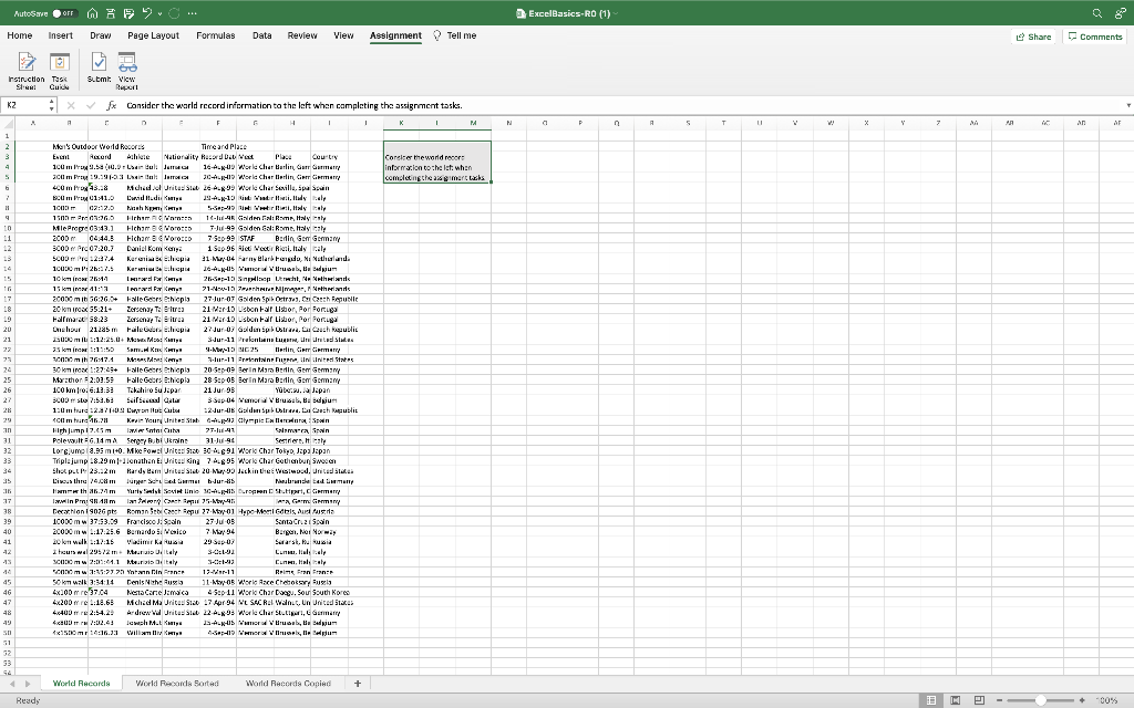
1	4	Insert a new column between columns B and C. Label the new column (cell C3) "Record ID"
2	4	Use the "Fill" feature of Excel to insert the numbers 1 to 47 in cells C4:C50.
3	2	Make the table headers (range B3:J3) bold
4	2	Center the table headers (range B3:J3) horizontally
5	2	Make cell B2 bold
6	2	Italizice cell B2
7	2	Make cell G2 bold
8	2	Italizice cell G2
9	4	Merge and center cell G2 across columns G:J
10	2	Change the format of the date range (G4:G73) to "Short Date"
11	2	Resize column B to a width of 28.0 (2.4 inches)
12	2	Resize column C to 8.71 (.79 inches)
13	2	Resize column D to 16.57 (1.44 inches)
14	2	Resize column E to 29.43 (2.53 inches) -notice this is smaller than needed to fit all cell contents
15	2	Resize column F to 15.14 (1.33 inches)
16	2	Resize column G to 11.0 (.99 inches)
17	2	Resize column H to 25.86 (2.22 inches)
18	2	Resize column I to 29.14 (2.5 inches)
19	2	Resize column J to 13.71 (1.21 inches)
20	4	Center the cells in the table (range B4:J50) horizontally
21	3	Notice that both the "Place" and "Country" fields display the country where the record was established. Hide column I ("Place") to avoid redundency in the table.
22	2	Place a "Thick Bottom Border" (from the border drop-down menu) under the data labels (range B3:J3)
23	5	Place a dotted line border (the option directly under "None" in the "Border" tab of the "Format Cells" dialog window) under each subsequent row in the table.
24	3	Fill rows 2 and 3 of the table (range B2:J3) using any color (not "No Fill") from the "Fill Color" drop-down menu.
25	5	Use the "Wrap Text" feature in Excel to display all of the contents of cells E46:E50. Resize the rows if necessary to fit the contents of the cells.
26	4	Set the print area of the worksheet to include only the area of the data table (Range B2:J50)
27	4	Set the left and right print margins of the worksheet to be .5 inches
28	3	Set column B as "Columns to repeat at left" page titles
29	3	Notice that there is a blank worksheet in the workbook named "World Records Copied". Navigate to that worksheet and select cell A1 if it is not already selected.
30	4	Copy the records table without row 2 (range B3:J50 from the "World Records" worksheet) to the "World Records Copied" worksheet using the "Copy" and "Paste" features of Excel. Paste the range starting in cell B3 of the "World Records Copied" worksheet.
31	8	Now, sort the table on the "World Records Sorted" worksheet by Country in ascending order (A to Z), then sort the table by 'Record Date' in descending order (Newest to Oldest).
32	8	Filter the table on the "World Records Sorted" worksheet to display only athletes whose "Nationality" listed as "Kenya" or "Jamaica"