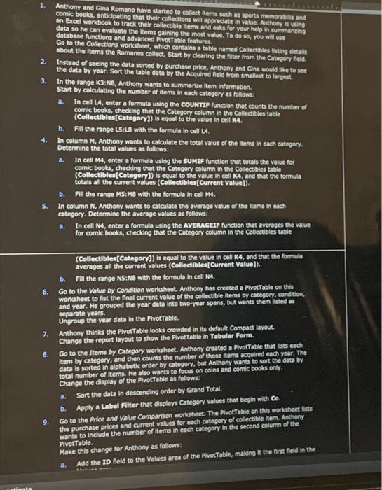
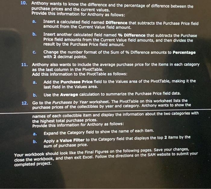
1. Anthony and Gina Romano have started to collect items such as sports memorabili and comic bools, anticipating that their collections will appreclate in value. Anthory is using. an Excel workbook to track their collectble items and asks for your help in wummartaing data so he can evaluate the items gaining the most value. To do so, you will use database functions and advanced PivotTable features. Ge to the Collections worksheet, which contains a table named Collectibles Eraing detally about the items the Romanos cellect start by clearing the fiter from the Category field. 2. Instead of seeing the data sorted by purchase price, Anthony and Cine would tave to see the data by year. Sort the table data by the Acquired field from smallest to largeat. 3. In the range KB :NB, Anthony wants to summarixe item information. Start by calculating the number of items in each category as follows: a. In cell L4, enter a formula uing the couNTIP function that counts the number of comic books, cheoking that the Category column in the Collectibles table (Collectibles[Category]) is equal to the value in cell K4. b. Fill the range 15 : L8 with the formula in cell LA. 4. In column M, Anthony wants to calculate the total value of the items in each category. Determine the total values as follows: a. In cell M4, enter a formula using the SuMrF function that totais the value for comic books, cheding that the Category column in the Collectibles table (Collectlblea[Category]) is equal to the value in cell XA, and that the formula totals all the current values (Collectblesf(Current Value]). b. Fill the range MS: M8 with the formula in cell M4. 5. In column N, Anthony wants to calculate the average value of the ltems in each category, Determine the average values as follows: a. In cell N4, enter a formula using the AVEAMGErF function that avereges the value for comic books, checking that the Category column in the Collectbies table (Collectibles[Category]) is equal to the value in cell K4, and that the formula avereges all the current values (Collectibles[Current Value]). b. Fill the range NS:NS with the formula in cell N4. 6. Go to the Value by Condivon worksheet. Anthony has created a PivotTable on this worksheet to list the final current value of the collectble items by category, condidion, and year. He grouped the year data into two-year spans, but wants them listed as separate years. Ungroup the year data in the PivotTable. 7. Anthony thinks the PivotTable looks crowded in lts default Compact layout. Change the report layout to show the PlvotTable in Tabular Form. 8. Go to the Jtems by Category worksheet. Anthony created a PlvotTable that lats each item by category, and then counts the number of those ltems acquired each year. The data is sorted in alphabetic order by category, but Anthony wants to sort the data by total number of items. He also wants to focus on coins and comic books only. Change the display of the Pivottable as follows: 3. Sort the date in descending order by Grand Total. b. Apply a Label Fitter that displays Category values that begin with Co. 9. Go to the Price and Value Comparison worksheet. The PivotTable on this worlaheet lists the purchase prices and current values for each category of collectible item. Anthony whe purchase prices and current include the number of items in each category in the second column of the Pivottable. Make this change for Anthony as follows: a. Add the TD field to the Values area of the PivotTable, making it the first feld in the purchase prices and the current values. Provide this information for Anthony as follows: a. Insert a calculated field named Difference that subtracts the Purchase Price field amount from the Current Value field amount. b. Insert another calculated field named \% Difference that subtracts the Purchase Price field amounts from the Current Value field amounts, and then divides the result by the Purchase Price field amount. c. Change the number format of the Sum of \% Difference amounts to Percentage with 2 decimal points. 11. Anthony also wants to include the average purchase price for the items in each category as the last column in the PivotTable. Add this information to the PivotTable as follows: a. Add the Purchase Price field to the Values area of the PivotTable, making it the last field in the Values area. b. Use the Average calculation to summarize the Purchase Price field data. 12. Go to the Purchases by Year worksheet. The PivotTable on this worksheet lists the purchase prices of the collectibles by year and category. Anthony wants to show the names of each collectible item and display the information about the two categories with the highest total purchase prices. Provide this information for Anthony as follows: a. Expand the Category field to show the name of each item. b. Apply a Value Fitter to the Category field that displays the top 2 items by the sum of purchase price. our workbook should look like the Final Figures on the following pages. Save your changes, ose the workbook, and then exit Excel. Follow the directions on the SAM website to submit your ompleted project


