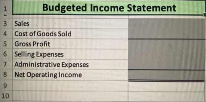
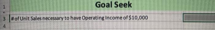
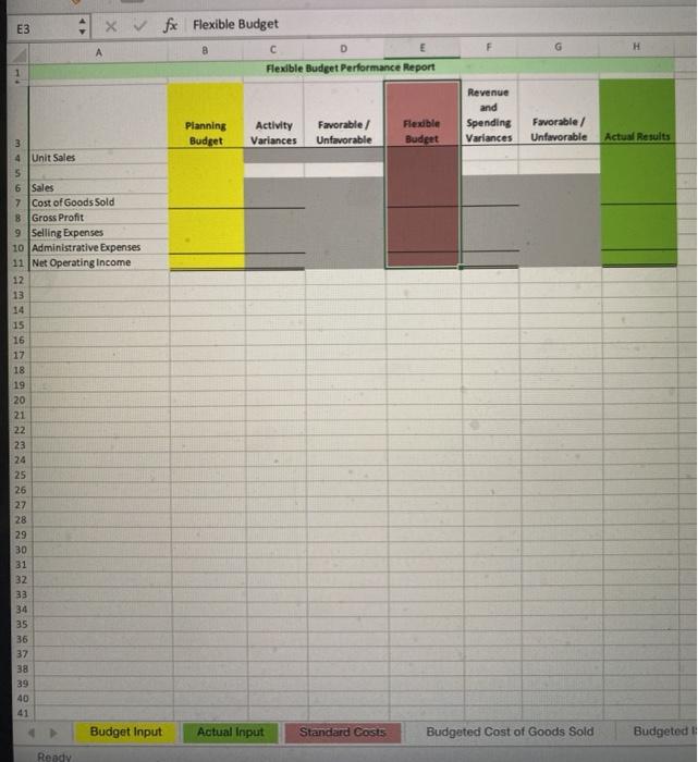
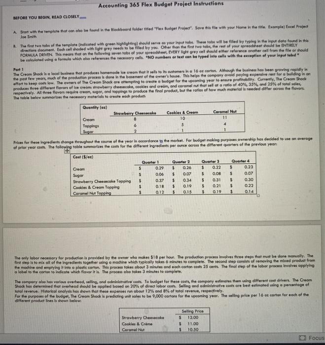
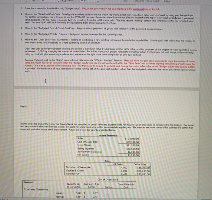
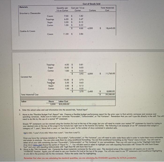
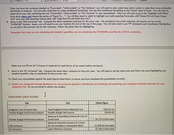
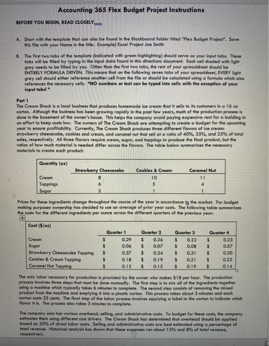
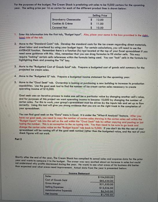
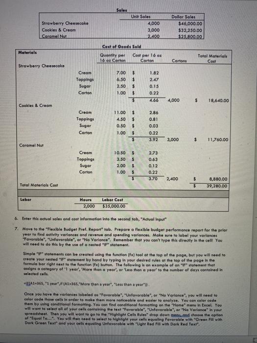
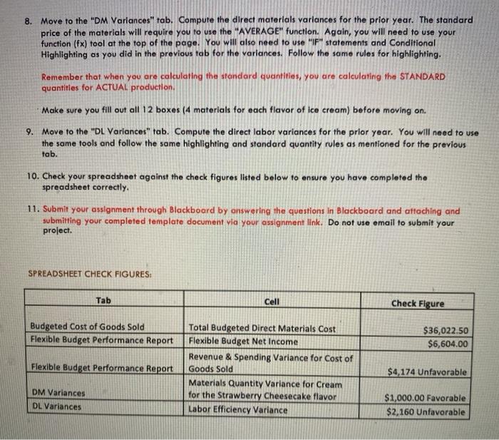
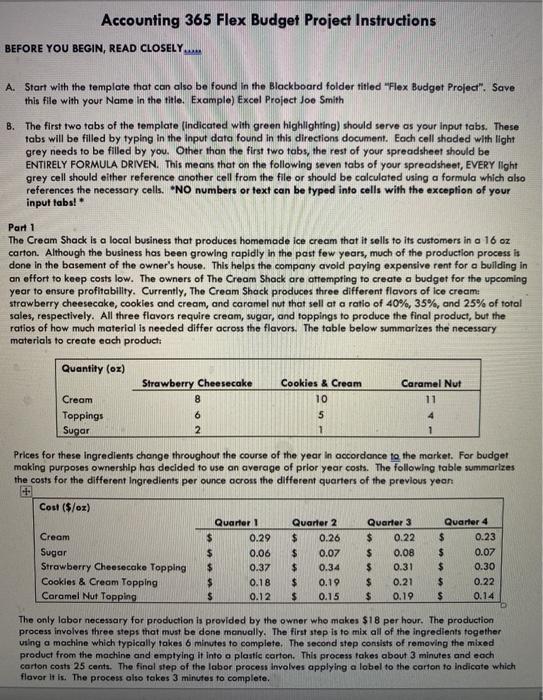
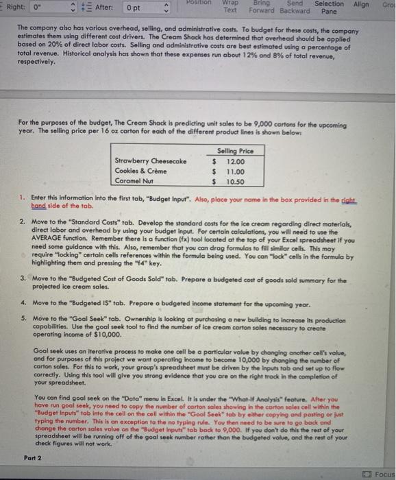
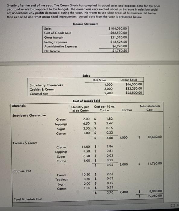
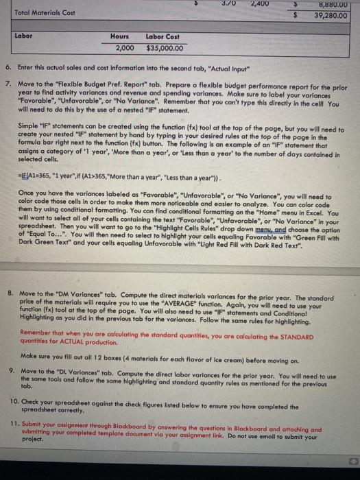
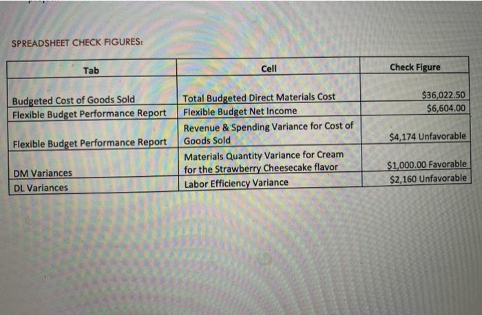
1 Budgeted Income Statement 3 Sales 4 Cost of Goods Sold 5 Gross Profit 6 Selling Expenses 7 Administrative Expenses 8 Net Operating Income 9 10 Goal Seek 1 3 # of Unit Sales necessary to have Operating Income of $10,000 4 4 E3 fx Flexible Budget 8 c D Flexible Budget Performance Report Revenue and Spending Variances Planning Budget Activity Variances Favorable/ Unfavorable Flexible Budert Favorable/ Unfavorable Actual Results 3 4 Unit Sales 5 6 Sales 7 Cost of Goods Sold 8 Gross Profit 9 Selling Expenses 10 Administrative Expenses 11 Net Operating Income 12 13 15 16 17 18 19 20 21 22 23 24 25 26 27 28 29 30 31 32 33 34 35 36 37 38 39 40 41 Budget Input Actual Input Standard Costs Budgeted Cost of Goods Sold Budgeted! Ready Accounting 365 Flex Budget Project Instructions BEFORE YOU BEGIN, READ CLOSELY A Start with the template that can also be found in the Blackboard folder titled "Flex Budget Project". Seve this file with your Non the title Example) Excel Project Joe Smith * The first two tobe of the template (indicated with green highlighting) should serve as your input tabs. These tobe will be filled by typing in the input data found in this dredion document. Each cell shaded with light grey needs to be filled by you. Other than the first two fobs, the rest of your spreadsheet should be ENTIRELY FORMULA DRIVEN. This means that on the following seven tobs of your spreadsheet, EVERY light grey cel should alther reference another call from the file or should be calculated using a formula which also references the necessary cells. "NO numbers or text can be typed into calls with the exception of your input fubd Part 1 The Cream Shook is a local business that produces homemade ice cream that it sel to its customen ha 16 or carton. Although the business has been growing rapidly in the past few years, much of the production process is done in the basement of the owner's house. This helps the company avoid paying expensive rent for a building in on effort to keep costs low. The owner of The Cream Shock are attempting to create a budget for the upcoming year to ensure profitability. Currently, The Cracom Shock produces three different flavors of ice cream strawberry Cheesecake, cookies and cream, and caramel rut that sell of a ratio of 40%, 35% and 25% of total soles, respectively. All three flavors require cream, sugar, and toppings to produce the final product, but the ratio of how much material is needed differ scrow the flavor The table below summarizes the necessary materials to create each product Quantity (er) Strawberry Cheesecake Cream Toppings Sugar Cookies & Cream 10 5 1 Caramel Nur 11 4 1 2 Prices for these ingredients change throughout the course of the year in occordance to the market. For budget moking purposes ownership has decided to use on average of prior year costs. The following toble summarizes the costs for the different ingredients per ounce across the different quarters of the previous yeon Cost (5/0x) Cream Sugar Strawberry Cheesecake Topping Cookies & Cream Topping Caramel Nut Topping Quarter 1 $ 0.29 $ 0.06 $ 0.37 $ 0.18 $ 0.12 Quarter 2 $ 0.26 $ 0.07 $ 0.34 $ 0.19 5 0.15 Quarter 3 $ 0.22 $ 0.08 $ 0.31 $ 0.21 $ 0.19 Quarter 4 $ 0.23 $ 0.07 $ 0.30 $ 0.22 $ 0.14 The only labor necessary for production is provided by the owner who makes $18 per hour. The production process involves three steps that must be done manually. The first step is to mix all of the ingredients together using a machine which typically takes 6 minutes to complete. The second step consists of removing the mixed product from the machine and emptying it into a plastic carton. This process fokes obout 3 minutes and each carton costs 25 cents. The final step of the labor process involves applying a label to the carton to indicate which flavor it is. The process also takes 3 minutes to complete. The company also hos various overhead, selling, and administrative costs. To budget for these cort, the company estimates them using different cout drivent. The Cream Shock has determined that overhod should be applied based on 20% of direct loborcom. Selling and administrative coils are best estimated using a percentage of total revenue. Historical analysis has shown that these expenses run about 12% and 8% of total revenue, respectively. For the purposes of the budget, The Geam Shock la predicting witsoles to be 9,000 cartons for the upcoming year. The selling price per 16 or carton for each of the different product lines is shown below Strawberry Cheesecake Cookies & Creme Coromal Nut Selling Price $ 12.00 $ 11.00 $ 10.50 Focus Tek Forward Backward Pane 1. Enter this information to the first to, "Budget Inpur". Also, place your on the box provided in the data wide of the tob. 2. Move to the Standard Codetab. Develop the standard cont for the ice cream regarding direct material, direct lobor and overhead by using your budget Input For carton collations, you will need to use the AVERAOE fundon. Remember there is a function () ol located of the top of your Excel spreadsheet f you need some guidance with Also, remember that you can drog formules to fill similar cells. This may require locking certain cells references within the formule being wed. You can lock"calls the formulo by Nighting them and pressing the way. 3. Move to a "budgeted Cast of Goods Sold" tob. Prepare a budgeted cont of goods sold summary for the projected lee cream volen 4. Move to the "Budgeted IS" tob. Prepare a budgeted Income statene for the upcoming year 5. Move to the "Gool See tab. Ownership is booking of purchasing a new buteling to be 010 he production capabilities. Use the good work tool to find the number of le crom cortonsoles necessary to create operating income of $10,000 Goal soek vies on iterative process to make one call be a partir volve by changing other cell's volue, and for suport of the project we want operering income to become 10,000 by changing the number of cotton solat For this to work, your group's spreadsheet muut be driven by the inputs fob and set up to flow correctly. Using this tool will give you long evidence that you are on the right track in the completion of your spreadsheet. You can find goolveek on the "Dato mer in Excel is under the "Who- Anolyolefcture. After you have in golak, you need to copy the number of carton toles showing the carton sales cell within the "Budget puls" tab Wo the call on the cell with the Good Seek tot by the copying and powing of typing the sumber. The son exception to the typing rule You thanned to be sure to go back and change the carton las volia on the Budget to book - 9,000, you don't do the the rest of your preacher will be wing off of the goolseskrumber rather than the budgeted value and the rest of your hedefigures will work I Part 2 Shortly after the end of the year, The Crom Shock has compiled in actual tolerond expense dote for the prior year and works to compare it to the budget. The owner was very excited about an increase in wes but could not understand whyprolins decreased during the year. He woods to see what areas of wis bushe did better than expected and what oras med improvement Advol done from the year la presented below Income Statement Soles $104,050.00 Colf of Goods Sold 582,530.00 Gross Margin 321,520.00 Seling Experts 513,526,50 Adminle Expenses $6,243.00 Nel nome 51.750.50 Sales Unit Soler Dellor soles Strawberry Cheesecake 4,000 $46,000.00 Cookies & Cream 3,000 $32,250.00 Carane Nur 2.400 $25,800.00 Materials Quoni per 16 o Corton Cost of Goods Sold Cost per 16 1 Total Materials Carto Cartons Cout Strawberry Cheesecake Cream Toppings 7.00 5 6.505 1.82 2:47 Materials Quantity per 16 on Carton Cost of Goods Sold Cost per 10 or Total Materials Carton Cartons Cout Strawberry Cheesecake Cream Toppings Sugar Carton 7.00 $ 6.50 $ 2.50 $ 1.00 $ 5 1.82 2.47 0.15 0.22 4.68 4,000 $ 18,640.00 Cookies & Cream Creom 11.00 $ 286 Toppings Sugar Carton 4.50 $ 0.50 $ 1.00 $ 5 0.81 0.03 0.22 392 3,000 $ 11,760.00 Caramel Nut Cream Toppings Sugor Corton 10.50 $ 3.50 $ 2.00 $ 1.00 $ 13 2.73 0.63 0.12 022 370 2,400 3,830.00 39,280.00 Total Materials Cost Labor Hours Labor Cout 2,000 $35,000.00 6. Enter this actual sales and cont Information into the second rob, "Actual pur 7. Move to the Flexible Budget Pret. Report" sob. Prepare a flexible budget performance report for the prior year to find activity variances and revenue and pending varianter. Make sure to lobel your variances "Favorable "Unfavorable", or "No Vorlance Remember that you can'type the directly in the call you will need to do this by the wie of a nested statement. Simple statements can be created using the function (ta) tool at the top of the page, but you will need to create your nested statement by hand by typing in your desired rules of the top of the page in the formula barrior next to the function (x) button. The following is an example of on statement that anima category of year', 'More than a year, or "Less than a year to the number of days contained in Heleded cell HEAT 365, 1 yearf (A1>365, "More than a year, less than a year Once you have the variances labeled or "Favorable", "Unfavorable or "No Variance, you will need to color code thone calls in order to make them more nericeable and easier to analyze. You can color code them by using conditional formatting, you can find conditional formatting on the "Home" menu in Excel You will want to select all of your cells containing the text favorable" Unfavorable"or "No Varlonce in your spreadsheet. Then you will want to go to the Highlight Cell Rules" drop down choose the option of Equal To. You will then need to select to Wohh your collequeling Favorable with "Green Fill with Dark Green Texe" and your cell equoling Unfavorable with Light Red with Dark Red Text 8. Move to the DM Vorlancas" tab. Compute the direct material variance for the prior year. The standard price of the material will require you to use the PAVERAGE function. Agory you will need to use your function(x) fool at the top of the page. You will also need to use "P" teman and Conditional High ing at you did in the previous tob for the Vorlonces Follow the same rules for highlighting Remember that when you are calculating the standard quarter you are calculating the STANDARD quarties for ACTUAL production HR DALWdro dile Once you have the variances labeled as "Favorable", "Unfavorable", or "No Vorlonce", you will need to color code those colls in order to make them more noticeable and easier to analyze. You can color code them by using conditional formatting. You can find conditional formatting on the "Homo" menu in Excel. You will want to select all of your cells containing the text "Favorable", "Unfavorable", or "No Variance in your spreadsheet. Then you will want to go to the "Highlight Colls Rules" drop down men and choose the option of "Equal To...". You will then need to select to highlight your cells equaling Favorable with "Green Fill with Dark Green Text" and your cells equaling Unfavorable with light Red Fill with Dark Red Text 8. Move to the "DM Variances" tob. Compute the direct materials variances for the prior year. The standard price of the materials will require you to use the "AVERAGE" function. Again, you will need to use your function (fx) tool of the top of the page. You will also need to use "P" statements and Conditional Highlighting as you did in the previous tab for the variances. Follow the same rules for highlighting. Remember that when you are colculorna the standard quartiles, you are collerine the STANDARD quantities for ACTUAL production Make sure you fill out all 12 boxes (4 materials for each flavor of ice cream) before moving on. 9. Move to the "DL Vorlonces" tab. Compute the direct labor vorlances for the prlor year. You will need to use the same tools and follow the same highlighting and standard quantity rules as mentioned for the previous tab. 10. Check your spreadsheet against the check figures thated below to ensure you have completed the spreadsheet correctly 11. Submit your assignment through Blackboard by answering the questions in Boekhoord ond ohlaching and submitting your completed templare document via your augment link. Do not use email to submit your project I SPREADSHEET CHECK FIGURES Tab Cell Check Figure Budgeted Cost of Goods Sold Flexible Budget Performance Report $36,022.50 $6,604.00 Flexible Budget Performance Report Total Budgeted Direct Materials Cost Flexible Budget Net Income Revenue & Spending Variance for Cost of Goods Sold Materials Quantity Variance for Cream for the Strawberry Cheesecake flavor Labor Efficiency Variance $4,174 Unfavorable DM Variances DL Variances $1,000.00 Favorable $2.160 Unfavorable Accounting 365 Flex Budget Project Instructions BEFORE YOU BEGIN, READ CLOSELY..... A. Start with the template that can also be found in the Blackboard folder titled "Flex Budget Project". Sove this file with your Nome in the title Example) Excel Project Joe Smith 8. The first two tabs of the template (indicated with green highlighting) should serve as your input tabs. These tabs will be filled by typing in the input data found in this directions document. Each cell shaded with light grey needs to be filled by you. Other than the first two tabs, the rest of your spreadsheet should be ENTIRELY FORMULA DRIVEN. This means that on the following seven tabs of your spreadsheet, EVERY light grey cell should either reference another cell from the file or should be calculated using a formula which also references the necessary cells. "NO numbers or text can be typed into cells with the exception of your input tebal Part 1 The Cream Shack is a local business that produces homemade ice cream that it sells to its customers in a 16 oz carton. Although the business has been growing rapidly in the past few years, much of the production process is done in the basement of the owner's house. This helps the company avoid paying expensive rent for a building in an effort to keep costs low. The owners of The Cream Shack are attempting to create a budget for the upcoming year to ensure profitability. Currently, The Cream Shock produces three different flavors of ice cream strawberry cheesecake, cookles and cream, and caramel nut that sell at a ratio of 40%, 35%, and 25% of total sales, respectively. All three flavors require cream, sugar, and toppings to produce the final product, but she ratios of how much material is needed differ across the flavors. The table below summarizes the necessary materials to create each product Quantity (or) Strawberry Cheesecake Cookies & Cream 10 5 Caramel Nut 11 Cream Toppings Sugar 6 2 Prices for these ingredients change throughout the course of the year in accordance to the market. For budget moking purposes ownership has decided to use an average of prior year costs. The following table summarizes the costs for the different ingredients per ounce across the different quarters of the previous year Cost ($/ox) Cream Sugar Strawberry Cheesecake Topping Cookies & Cream Topping Caramel Nut Topping Quarter 1 5 0.29 $ 0.06 $ 0.37 $ 0.18 $ 0.12 Quarter 2 $ 0.26 $ 0.07 $ 0.34 $ 0.19 $ 0.15 Quarter 3 $ 0.22 $ 0.08 $ 0.31 $ 0.21 $ 0.19 Quarter 4 $ 0.23 $ 0.07 $ 0.30 $ 0.22 $ 0.14 The only labor necessary for production is provided by the owner who makes $18 per hour. The production process involves three steps that must be done manually. The first step is to mix all of the ingredients together using a machine which typically takes 6 minutes to complete. The second step consists of removing the mixed product from the machine and emptying it into a plastic carton. This process tokes about 3 minutes and each carton costs 25 cents. The final step of the labor process involves applying a label to the carton to indicate which flavor it. The process also tokes 3 minutes to complete. The company also has various overhead, telling, and administrative costs. To budget for these costs, the company estimates them using different cost drivers. The Cream Shock has determined that overhead should be applied based on 20% of direct labor costs. Selling and administrative costs are best estimated using a percentage of total revenue. Historical analysis has shown that these expenses run about 12% and 8% of total revenue, respectively. For the purposes of the budget, The Cream Shack is predicting unit sales to be 9,000 cartons for the upcoming year. The selling price per 16 oz carton for each of the different product lines is shown below: Strawberry Cheesecake Cookies & Creme Caramel Nut Selling Price $ 12.00 $ 11.00 $ 10.50 1. Enter this information into the first tab, "Budget Input". Also, place your name in the box provided in the doht. hand side of the tab. 2. Move to the Standard Cosht" tab. Develop the standard costs for the ice cream regarding direct materials, direct labor and overhead by using your budget input. For certain calculations, you will need to use the AVERAGE function. Remember there is a function (x) tool located at the top of your Excel spreadsheet If you need some guidance with this. Also, remember that you can drag formules to fill similar cells. This may require locking certain cells references within the formula being used. You can lock" cells in the formulo by Highlighting them and pressing the "44"key. 3. Move to the "Budgeted Coat Goods Sold" tab. Prepare a budgeted cost of goods sold summary for the projected ice cream sales. 4. Move to the "Budgeted IS" tab. Prepare a budgeted income statement for the upcoming year. 5. Move to the "Goal Seek" tab. Ownership is looking at purchasing a new building to Increase its production capabilities. Use the goal seek tool to find the number of ice cream carton sales necessary to create operating Income of $10,000. Goal seakuses on iterative process to make one cell be a particular value by changing another call's value, and for purposes of this project we want operating income to become 10,000 by changing the number of carton sale. For this to work, your group's spreadsheet must be driven by the Inputs tab and set up to flow correctly. Using this tool will give you strong evidence that you are on the right track in the completion of your spreadsheet. You can find goal seek on the "Data" menu In Excel. It is under the "What-If Analysis" feature. After you have run goal seek, you need to copy the number of carton sales showing in the carton soles cell within the "Budget Inputs" tob Into the call on the cell within the "Gool Seek" tab by alther copying and pasting or at typing the number. This is an exception to the notyping rule. You then need to be sure to go back and change the carton tales value on the "Budget Inputs" tab back to 9,000. If you don't do this the rest of your spreadsheet will be running off of the goal seek number rather than the budgeted value, and the rest of your check figures will not work. Part 2 Shortly after the end of the year, The Cream Shack has compiled its actual sales and expense data for the prior year and wants to compare it to the budget. The owner was very excited about an increase in sales but could not understand why profit decreased during the year. He wants to see what areas of his business did better than expected and what areas need improvement. Actual data from the year la presented below Income Statement Soles $104,050.00 Cost of Goods Sold $82 530.00 Grou Margin $21,520.00 Selling Expenses $13,526.50 Administrative Experts $6,243.00 Net Income 51 750.50 Sales Strawberry Cheesecake Cookies & Cream Caramel Nut Unit Sales 4,000 3,000 2.400 Dollar Sales $46,000.00 $32,250.00 $ 25,800.00 Materials Cast of Goods Sold Quantity per Cost per 16 oz 16 oz Carton Carton Total Materials Cost Cartons Strawberry Cheesecake $ $ Cream Toppings Sugar Carton 7.00 6.50 2.50 1.00 1.82 2.47 0.15 0.22 $ $ $ 4.66 4,000 $ 18,640.00 Cookies & Cream $ $ Cream Toppings Sugar Carton 11.00 4.50 0.50 1.00 2.86 0.81 0.03 $ $ $ 0.22 3.92 3,000 $ 11,760.00 Caramel Nut Cream Topping: Sugar Carton 10.50 3.50 2.00 1.00 $ $ $ $ $ 2.73 0.63 0.12 0.22 3.70 2,400 $ $ 8,880.00 39,280.00 Total Materials Cout Labor Hours 2,000 Labor Cost $35,000.00 6. Enter this actual sales and cost Information into the second tob, "Actual Input" 7. Move to the "Flexible Budget Pref. Report" tab. Prepare a flexible budget performance report for the prior year to find activity variances and revenue and spending variances. Make wre to label your variances "Favorable". "Unfavorable", or "No Variance". Remember that you can't type this directly in the celll You will need to do this by the use of a nested IF statement. Simple "F" statements can be created using the function (x) tool at the top of the page, but you will need to create your nested "Matement by hand by typing in your desired rules at the top of the page in the formula bar right next to the function (fx] button. The following is an example of an "F" statement that ouigni a category of 'l year', 'More than a year, or less than a year to the number of days contained in selected cells UA365, 1 year Al>365,"More than a year". "Less than a year")) Once you have the varlonces labeled as "Favorable", "Unfavorable", or "No Variance, you will need to color code those cells in order to make them more noticeable and easier to analyze. You can color code them by using conditional formatting. You can find conditional formatting on the "Home" menu in Excel. You will want to select all of your colle containing the text "Favorable". "Unfavorable", or "No Variance in your spreadsheet. Then you will want to go to the "Highlight Cells Rules" dro down me and choose the option of "Equal To..." You will then need to select to highlight your cell equaling Favorable with Green Fill with Dark Green Text" ond your cell equaling Unfavorable with light Red Pill with Dark Red Text". 8. Move to the "DM Variances" tab. Compute the direct materials variances for the prior year. The standard price of the materials will require you to use the "AVERAGE" function. Again, you will need to use your function (fx) tool at the top of the page. You will also need to use "F" statements and Conditional Highlighting as you did in the previous tab for the variances. Follow the same rules for highlighting. Remember that when you are calculating the standard quantities, you are calculating the STANDARD quantities for ACTUAL production, Make sure you fill out all 12 boxes (4 materials for each flavor of ice cream) before moving on. 9. Move to the "DL Variances" tab. Compute the direct labor varlances for the prior year. You will need to use the same tools and follow the same highlighting and standard quantity rules as mentioned for the previous tab. 10. Check your spreadsheet against the check figures listed below to ensure you have completed the spreadsheet correctly. 11. Submit your assignment through Blackboard by onswering the questions in Blackboard and attaching and submitting your completed template document via your assignment link. Do not use email to submit your project. SPREADSHEET CHECK FIGURES: Tab Cell Check Figure Budgeted Cost of Goods Sold Flexible Budget Performance Report $36,022.50 $6,604.00 Flexible Budget Performance Report Total Budgeted Direct Materials Cost Flexible Budget Net Income Revenue & Spending Variance for Cost of Goods Sold Materials Quantity Variance for Cream for the Strawberry Cheesecake flavor Labor Efficiency Variance $4,174 Unfavorable DM Variances DL Variances $1,000.00 Favorable $2,160 Unfavorable Accounting 365 Flex Budget Project Instructions BEFORE YOU BEGIN, READ CLOSELY A. Start with the template that can also be found in the Blackboard folder titled "Flex Budget Project". Save this file with your Name in the title. Example) Excel Project Joe Smith 8. The first two tabs of the template (indicated with green highlighting) should serve as your input tabs. These tabs will be filled by typing in the input data found in this directions document. Each cell shaded with light grey needs to be filled by you. Other than the first two tabs, the rest of your spreadsheet should be ENTIRELY FORMULA DRIVEN. This means that on the following seven tabs of your spreadsheet, EVERY light grey cell should either reference another cell from the file or should be calculated using a formula which also references the necessary cells. *NO numbers or text can be typed into cells with the exception of your input tabs! Part 1 The Cream Shack is a local business that produces homemade ice cream that it sells to its customers in a 16 oz carton. Although the business has been growing rapidly in the past few years, much of the production process is done in the basement of the owner's house. This helps the company avold paying expensive rent for a building in an effort to keep costs low. The owners of The Cream Shack are attempting to create a budget for the upcoming year to ensure profitability. Currently, The Cream Shack produces three different flavors of ice cream strawberry cheesecake, cookies and cream, and caramel nut that sell at a ratio of 40%, 35%, and 25% of total sales, respectively. All three flavors require cream, sugar, and toppings to produce the final product, but the ratios of how much material is needed differ across the flavors. The table below summarizes the necessary materials to create each product: Quantity (oz) Cream Toppings Sugar Strawberry Cheesecake 8 6 2 Cookies & Cream 10 5 1 Caramel Nut 11 4 Prices for these ingredients change throughout the course of the year in accordance to the market. For budget making purposes ownership has decided to use an average of prior year costs. The following table summarizes the costs for the different Ingredients per ounce across the different quarters of the previous yeon Cost ($/ox) Cream Sugar Strawberry Cheesecake Topping Cookies & Cream Topping Caramel Nut Topping Quarter 1 0.29 $ 0.06 $ 0.37 $ 0.18 $ 0.12 Quarter 2 $ 0.26 $ 0.07 $ 0.34 $ 0.19 $ 0.15 Quarter 3 $ 0.22 $ 0.08 $ 0.31 $ 0.21 $ 0.19 Quarter 4 $ 0.23 $ 0.07 $ 0.30 $ 0.22 $ 0.14 The only labor necessary for production is provided by the owner who makes $18 per hour. The production process involves three steps that must be done manually. The first step is to mix all of the ingredients together ving a machine which typically takes 6 minutes to complete. The second step consists of removing the mixed product from the machine and emptying it into a plastic carton. This process takes about 3 minutes and each carton costs 25 cents. The final step of the labor process involves applying a label to the carton to indicate which flavor it is. The process also takes 3 minutes to complete. Right: 0 Position After: O pt Wrap Text Being Send Forward Backward Selection Pane Align Groe The company also has various overhead, selling, and administrative costs. To budget for these costs, the company estimates them using different cost drivers. The Cream Shock has determined that overhead should be applied based on 20% of direct labor costs. Selling and administrative couts are best estimated using a percentage of total revenue. Historical analysis has shown that these expenses run about 12% and 8% of total revenue, respectively, For the purposes of the budget, The Cream Shack is predicting unit sales to be 9,000 cartons for the upcoming year. The selling price per 16 oz corton for each of the different product lines is shown below Selling Price Strawberry Cheesecake $ 12.00 Cookies & Creme $ 11.00 Caramel Nut $ 10.50 1. Enter this information into the first tab, "Budget Input". Also, place your name in the box provided in the tight hand side of the tob. 2. Move to the Standard Costs" tab. Develop the standard costs for the ice cream regarding direct materials, direct labor and overhead by using your budget input. For certain calculations, you will need to use the AVERAGE function. Remember there is a function (fx) tool located at the top of your Excel spreadsheet If you need some guidance with this. Also, remember that you can drag formulas to fill similor cells . This may require "locking certain cells references within the formula being used. You can lock" cells in the formula by highlighting them and pressing the "14"key. 3. Move to the "Budgeted Cost of Goods Sold" tab. Prepare a budgeted cost of goods sold summary for the projected ice cream soles. 4. Move to the "Budgeted 15" tob. Prepare a budgeted Income statement for the upcoming year. 5. Move to the "Goal Seek" tab. Ownership is looking at purchasing a new building to Increase its production capabilities. Use the goal seek tool to find the number of ice cream carton soles necessary to create operating income of $10,000. Goal seek uses on Iterative process to make one cell be a particular value by changing another cel's volue, ond for purposes of this project we want operating income to become 10,000 by changing the number of carton sales. For this to work, your group's spreadsheet must be driven by the inputs tab and set up to flow correctly. Using this tool will give you strong evidence that you are on the right trock in the completion of your spreadsheet. You can find goal seek on the "Data" menu in Excel. It is under the "What If Analysis" feature. After you have run gool seek, you need to copy the number of carton sales showing in the carton soles cell within the "Budget Inputs" tob Into the cell on the cell within the "Gool Seek" tab by either copying and pasting or just typing the number. This is on exception to the no typing rule. You the need to be sure to go back and change the carton soles value on the Budget Input" tob back to 9,000. If you don't do this the rest of your spreadsheet will be running off of the goal seek number rather than the budgeted volue, and the rest of your check figures will not work. Part 2 HD Focus Shortly after the end of the year, The Cream Shack has compiled its actual sales and expense data for the prior year and wants to compare it to the budget. The owner was very excited about an increase in sales but could not understand why profits decreased during the year. He wants to see what areas of his business did better than expected and what areas need improvement. Actual data from the year is presented below Income Statement Sales $104,050.00 Cost of Goods Sold $82,530.00 Gross Margin $21,520.00 Selling Expenses $13,526.50 Administrative Expenses $6,243.00 Net Income $1750.50 Sales Strawberry Cheesecake Cookies & Cream Caramel Nut Unit Sales 4,000 3,000 2,400 Dollar Sales $46,000.00 $32,250.00 $25,800.00 Materials Cost of Goods Sold Quantity per Cost per 16 oz 16 oz Carton Carton Total Materials Cost Cartons Strawberry Cheesecake Cream Toppings Sugar Carton 7.00 6.50 2.50 1.00 $ $ $ $ $ 1.82 2.47 0.15 0.22 4.66 4,000 $ 18,640.00 Cookies & Cream Cream Toppings Sugar Carton 11.00 4.50 0.50 1.00 $ $ $ $ $ 2.86 0.81 0.03 0.22 3.92 3,000 $ 11,760.00 Caramel Nut Cream Toppings Sugar Carton 10.50 3.50 2.00 1.00 $ $ $ $ 2.73 0.63 0.12 0.22 3.70 $ 2,400 $ $ 8,880.00 39,280.00 Total Materials Cost 3.70 2,400 Total Materials Cost 8,880.00 39,280.00 $ Labor Hours 2,000 Labor Cost $35,000.00 6. Enter this actual sales and cost Information into the second tab, "Actual Input 7. Move to the "Flexible Budget Pref. Report" tab. Prepare a flexible budget performance report for the prior year to find activity variances and revenue and spending variances. Make sure to label your variances "Favorable", "Unfavorable", or "No Variance". Remember that you can't type this directly in the celll You will need to do this by the use of a nested "IP" statement. Simple "P" statements can be created using the function (fx) tool at the top of the page, but you will need to create your nested "F" statement by hand by typing in your desired rules at the top of the page in the formula bar right next to the function (fx) button. The following is an example of an "F" statement that assigns a category of '1 year', 'More than a year', or "Less than a year' to the number of days contained in selected cells. LE(A1-365, "1 year" if (A1>365,"More than a year", "Less than a year")). Once you have the variances labeled as "Favorable", "Unfavorable", or "No Variance", you will need to color code those cells in order to make them more noticeable and easier to analyze. You can color code them by using conditional formatting. You can find conditional formatting on the "Home" menu in Excel. You will want to select all of your cells containing the text "Favorable", "Unfavorable", or "No Variance" in your spreadsheet. Then you will want to go to the "Highlight Cells Rules" drop down menu, and choose the option of "Equal To...". You will then need to select to highlight your cells equaling Favorable with "Green Fill with Dark Green Text" and your cells equaling Unfavorable with "Light Red Fill with Dark Red Text". 8. Move to the "DM Varlances" tab. Compute the direct materials varlonces for the prior year. The standard price of the materials will require you to use the "AVERAGE" function. Again, you will need to use your function (fx) tool at the top of the page. You will also need to use "F" statements and Conditional Highlighting as you did in the previous tab for the variances. Follow the same rules for highlighting. Remember that when you are calculating the standard quantities, you are calculating the STANDARD quantities for ACTUAL production. Make sure you fill out all 12 boxes (4 materials for each flavor of ice cream) before moving on 9. Move to the "DL Variances" tab. Compute the direct labor variances for the prior year. You will need to use the same tools and follow the same highlighting and standard quantity rules os mentioned for the previous tab. 10. Check your spreadsheet against the check figures listed below to ensure you have completed the spreadsheet correctly. 11. Submit your assignment through Blackboard by answering the questions in Blackboard and attaching and submitting your completed template document via your assignment link. Do not use email to submit your project SPREADSHEET CHECK FIGURES: Tab Cell Check Figure Budgeted Cost of Goods Sold Flexible Budget Performance Report $36,022.50 $6,604.00 Total Budgeted Direct Materials Cost Flexible Budget Net Income Revenue & Spending Variance for Cost of Goods Sold Materials Quantity Variance for Cream for the Strawberry Cheesecake flavor Labor Efficiency Variance Flexible Budget Performance Report $4,174 Unfavorable DM Variances DL Variances $1,000.00 Favorable $2,160 Unfavorable 1 Budgeted Income Statement 3 Sales 4 Cost of Goods Sold 5 Gross Profit 6 Selling Expenses 7 Administrative Expenses 8 Net Operating Income 9 10 Goal Seek 1 3 # of Unit Sales necessary to have Operating Income of $10,000 4 4 E3 fx Flexible Budget 8 c D Flexible Budget Performance Report Revenue and Spending Variances Planning Budget Activity Variances Favorable/ Unfavorable Flexible Budert Favorable/ Unfavorable Actual Results 3 4 Unit Sales 5 6 Sales 7 Cost of Goods Sold 8 Gross Profit 9 Selling Expenses 10 Administrative Expenses 11 Net Operating Income 12 13 15 16 17 18 19 20 21 22 23 24 25 26 27 28 29 30 31 32 33 34 35 36 37 38 39 40 41 Budget Input Actual Input Standard Costs Budgeted Cost of Goods Sold Budgeted! Ready Accounting 365 Flex Budget Project Instructions BEFORE YOU BEGIN, READ CLOSELY A Start with the template that can also be found in the Blackboard folder titled "Flex Budget Project". Seve this file with your Non the title Example) Excel Project Joe Smith * The first two tobe of the template (indicated with green highlighting) should serve as your input tabs. These tobe will be filled by typing in the input data found in this dredion document. Each cell shaded with light grey needs to be filled by you. Other than the first two fobs, the rest of your spreadsheet should be ENTIRELY FORMULA DRIVEN. This means that on the following seven tobs of your spreadsheet, EVERY light grey cel should alther reference another call from the file or should be calculated using a formula which also references the necessary cells. "NO numbers or text can be typed into calls with the exception of your input fubd Part 1 The Cream Shook is a local business that produces homemade ice cream that it sel to its customen ha 16 or carton. Although the business has been growing rapidly in the past few years, much of the production process is done in the basement of the owner's house. This helps the company avoid paying expensive rent for a building in on effort to keep costs low. The owner of The Cream Shock are attempting to create a budget for the upcoming year to ensure profitability. Currently, The Cracom Shock produces three different flavors of ice cream strawberry Cheesecake, cookies and cream, and caramel rut that sell of a ratio of 40%, 35% and 25% of total soles, respectively. All three flavors require cream, sugar, and toppings to produce the final product, but the ratio of how much material is needed differ scrow the flavor The table below summarizes the necessary materials to create each product Quantity (er) Strawberry Cheesecake Cream Toppings Sugar Cookies & Cream 10 5 1 Caramel Nur 11 4 1 2 Prices for these ingredients change throughout the course of the year in occordance to the market. For budget moking purposes ownership has decided to use on average of prior year costs. The following toble summarizes the costs for the different ingredients per ounce across the different quarters of the previous yeon Cost (5/0x) Cream Sugar Strawberry Cheesecake Topping Cookies & Cream Topping Caramel Nut Topping Quarter 1 $ 0.29 $ 0.06 $ 0.37 $ 0.18 $ 0.12 Quarter 2 $ 0.26 $ 0.07 $ 0.34 $ 0.19 5 0.15 Quarter 3 $ 0.22 $ 0.08 $ 0.31 $ 0.21 $ 0.19 Quarter 4 $ 0.23 $ 0.07 $ 0.30 $ 0.22 $ 0.14 The only labor necessary for production is provided by the owner who makes $18 per hour. The production process involves three steps that must be done manually. The first step is to mix all of the ingredients together using a machine which typically takes 6 minutes to complete. The second step consists of removing the mixed product from the machine and emptying it into a plastic carton. This process fokes obout 3 minutes and each carton costs 25 cents. The final step of the labor process involves applying a label to the carton to indicate which flavor it is. The process also takes 3 minutes to complete. The company also hos various overhead, selling, and administrative costs. To budget for these cort, the company estimates them using different cout drivent. The Cream Shock has determined that overhod should be applied based on 20% of direct loborcom. Selling and administrative coils are best estimated using a percentage of total revenue. Historical analysis has shown that these expenses run about 12% and 8% of total revenue, respectively. For the purposes of the budget, The Geam Shock la predicting witsoles to be 9,000 cartons for the upcoming year. The selling price per 16 or carton for each of the different product lines is shown below Strawberry Cheesecake Cookies & Creme Coromal Nut Selling Price $ 12.00 $ 11.00 $ 10.50 Focus Tek Forward Backward Pane 1. Enter this information to the first to, "Budget Inpur". Also, place your on the box provided in the data wide of the tob. 2. Move to the Standard Codetab. Develop the standard cont for the ice cream regarding direct material, direct lobor and overhead by using your budget Input For carton collations, you will need to use the AVERAOE fundon. Remember there is a function () ol located of the top of your Excel spreadsheet f you need some guidance with Also, remember that you can drog formules to fill similar cells. This may require locking certain cells references within the formule being wed. You can lock"calls the formulo by Nighting them and pressing the way. 3. Move to a "budgeted Cast of Goods Sold" tob. Prepare a budgeted cont of goods sold summary for the projected lee cream volen 4. Move to the "Budgeted IS" tob. Prepare a budgeted Income statene for the upcoming year 5. Move to the "Gool See tab. Ownership is booking of purchasing a new buteling to be 010 he production capabilities. Use the good work tool to find the number of le crom cortonsoles necessary to create operating income of $10,000 Goal soek vies on iterative process to make one call be a partir volve by changing other cell's volue, and for suport of the project we want operering income to become 10,000 by changing the number of cotton solat For this to work, your group's spreadsheet muut be driven by the inputs fob and set up to flow correctly. Using this tool will give you long evidence that you are on the right track in the completion of your spreadsheet. You can find goolveek on the "Dato mer in Excel is under the "Who- Anolyolefcture. After you have in golak, you need to copy the number of carton toles showing the carton sales cell within the "Budget puls" tab Wo the call on the cell with the Good Seek tot by the copying and powing of typing the sumber. The son exception to the typing rule You thanned to be sure to go back and change the carton las volia on the Budget to book - 9,000, you don't do the the rest of your preacher will be wing off of the goolseskrumber rather than the budgeted value and the rest of your hedefigures will work I Part 2 Shortly after the end of the year, The Crom Shock has compiled in actual tolerond expense dote for the prior year and works to compare it to the budget. The owner was very excited about an increase in wes but could not understand whyprolins decreased during the year. He woods to see what areas of wis bushe did better than expected and what oras med improvement Advol done from the year la presented below Income Statement Soles $104,050.00 Colf of Goods Sold 582,530.00 Gross Margin 321,520.00 Seling Experts 513,526,50 Adminle Expenses $6,243.00 Nel nome 51.750.50 Sales Unit Soler Dellor soles Strawberry Cheesecake 4,000 $46,000.00 Cookies & Cream 3,000 $32,250.00 Carane Nur 2.400 $25,800.00 Materials Quoni per 16 o Corton Cost of Goods Sold Cost per 16 1 Total Materials Carto Cartons Cout Strawberry Cheesecake Cream Toppings 7.00 5 6.505 1.82 2:47 Materials Quantity per 16 on Carton Cost of Goods Sold Cost per 10 or Total Materials Carton Cartons Cout Strawberry Cheesecake Cream Toppings Sugar Carton 7.00 $ 6.50 $ 2.50 $ 1.00 $ 5 1.82 2.47 0.15 0.22 4.68 4,000 $ 18,640.00 Cookies & Cream Creom 11.00 $ 286 Toppings Sugar Carton 4.50 $ 0.50 $ 1.00 $ 5 0.81 0.03 0.22 392 3,000 $ 11,760.00 Caramel Nut Cream Toppings Sugor Corton 10.50 $ 3.50 $ 2.00 $ 1.00 $ 13 2.73 0.63 0.12 022 370 2,400 3,830.00 39,280.00 Total Materials Cost Labor Hours Labor Cout 2,000 $35,000.00 6. Enter this actual sales and cont Information into the second rob, "Actual pur 7. Move to the Flexible Budget Pret. Report" sob. Prepare a flexible budget performance report for the prior year to find activity variances and revenue and pending varianter. Make sure to lobel your variances "Favorable "Unfavorable", or "No Vorlance Remember that you can'type the directly in the call you will need to do this by the wie of a nested statement. Simple statements can be created using the function (ta) tool at the top of the page, but you will need to create your nested statement by hand by typing in your desired rules of the top of the page in the formula barrior next to the function (x) button. The following is an example of on statement that anima category of year', 'More than a year, or "Less than a year to the number of days contained in Heleded cell HEAT 365, 1 yearf (A1>365, "More than a year, less than a year Once you have the variances labeled or "Favorable", "Unfavorable or "No Variance, you will need to color code thone calls in order to make them more nericeable and easier to analyze. You can color code them by using conditional formatting, you can find conditional formatting on the "Home" menu in Excel You will want to select all of your cells containing the text favorable" Unfavorable"or "No Varlonce in your spreadsheet. Then you will want to go to the Highlight Cell Rules" drop down choose the option of Equal To. You will then need to select to Wohh your collequeling Favorable with "Green Fill with Dark Green Texe" and your cell equoling Unfavorable with Light Red with Dark Red Text 8. Move to the DM Vorlancas" tab. Compute the direct material variance for the prior year. The standard price of the material will require you to use the PAVERAGE function. Agory you will need to use your function(x) fool at the top of the page. You will also need to use "P" teman and Conditional High ing at you did in the previous tob for the Vorlonces Follow the same rules for highlighting Remember that when you are calculating the standard quarter you are calculating the STANDARD quarties for ACTUAL production HR DALWdro dile Once you have the variances labeled as "Favorable", "Unfavorable", or "No Vorlonce", you will need to color code those colls in order to make them more noticeable and easier to analyze. You can color code them by using conditional formatting. You can find conditional formatting on the "Homo" menu in Excel. You will want to select all of your cells containing the text "Favorable", "Unfavorable", or "No Variance in your spreadsheet. Then you will want to go to the "Highlight Colls Rules" drop down men and choose the option of "Equal To...". You will then need to select to highlight your cells equaling Favorable with "Green Fill with Dark Green Text" and your cells equaling Unfavorable with light Red Fill with Dark Red Text 8. Move to the "DM Variances" tob. Compute the direct materials variances for the prior year. The standard price of the materials will require you to use the "AVERAGE" function. Again, you will need to use your function (fx) tool of the top of the page. You will also need to use "P" statements and Conditional Highlighting as you did in the previous tab for the variances. Follow the same rules for highlighting. Remember that when you are colculorna the standard quartiles, you are collerine the STANDARD quantities for ACTUAL production Make sure you fill out all 12 boxes (4 materials for each flavor of ice cream) before moving on. 9. Move to the "DL Vorlonces" tab. Compute the direct labor vorlances for the prlor year. You will need to use the same tools and follow the same highlighting and standard quantity rules as mentioned for the previous tab. 10. Check your spreadsheet against the check figures thated below to ensure you have completed the spreadsheet correctly 11. Submit your assignment through Blackboard by answering the questions in Boekhoord ond ohlaching and submitting your completed templare document via your augment link. Do not use email to submit your project I SPREADSHEET CHECK FIGURES Tab Cell Check Figure Budgeted Cost of Goods Sold Flexible Budget Performance Report $36,022.50 $6,604.00 Flexible Budget Performance Report Total Budgeted Direct Materials Cost Flexible Budget Net Income Revenue & Spending Variance for Cost of Goods Sold Materials Quantity Variance for Cream for the Strawberry Cheesecake flavor Labor Efficiency Variance $4,174 Unfavorable DM Variances DL Variances $1,000.00 Favorable $2.160 Unfavorable Accounting 365 Flex Budget Project Instructions BEFORE YOU BEGIN, READ CLOSELY..... A. Start with the template that can also be found in the Blackboard folder titled "Flex Budget Project". Sove this file with your Nome in the title Example) Excel Project Joe Smith 8. The first two tabs of the template (indicated with green highlighting) should serve as your input tabs. These tabs will be filled by typing in the input data found in this directions document. Each cell shaded with light grey needs to be filled by you. Other than the first two tabs, the rest of your spreadsheet should be ENTIRELY FORMULA DRIVEN. This means that on the following seven tabs of your spreadsheet, EVERY light grey cell should either reference another cell from the file or should be calculated using a formula which also references the necessary cells. "NO numbers or text can be typed into cells with the exception of your input tebal Part 1 The Cream Shack is a local business that produces homemade ice cream that it sells to its customers in a 16 oz carton. Although the business has been growing rapidly in the past few years, much of the production process is done in the basement of the owner's house. This helps the company avoid paying expensive rent for a building in an effort to keep costs low. The owners of The Cream Shack are attempting to create a budget for the upcoming year to ensure profitability. Currently, The Cream Shock produces three different flavors of ice cream strawberry cheesecake, cookles and cream, and caramel nut that sell at a ratio of 40%, 35%, and 25% of total sales, respectively. All three flavors require cream, sugar, and toppings to produce the final product, but she ratios of how much material is needed differ across the flavors. The table below summarizes the necessary materials to create each product Quantity (or) Strawberry Cheesecake Cookies & Cream 10 5 Caramel Nut 11 Cream Toppings Sugar 6 2 Prices for these ingredients change throughout the course of the year in accordance to the market. For budget moking purposes ownership has decided to use an average of prior year costs. The following table summarizes the costs for the different ingredients per ounce across the different quarters of the previous year Cost ($/ox) Cream Sugar Strawberry Cheesecake Topping Cookies & Cream Topping Caramel Nut Topping Quarter 1 5 0.29 $ 0.06 $ 0.37 $ 0.18 $ 0.12 Quarter 2 $ 0.26 $ 0.07 $ 0.34 $ 0.19 $ 0.15 Quarter 3 $ 0.22 $ 0.08 $ 0.31 $ 0.21 $ 0.19 Quarter 4 $ 0.23 $ 0.07 $ 0.30 $ 0.22 $ 0.14 The only labor necessary for production is provided by the owner who makes $18 per hour. The production process involves three steps that must be done manually. The first step is to mix all of the ingredients together using a machine which typically takes 6 minutes to complete. The second step consists of removing the mixed product from the machine and emptying it into a plastic carton. This process tokes about 3 minutes and each carton costs 25 cents. The final step of the labor process involves applying a label to the carton to indicate which flavor it. The process also tokes 3 minutes to complete. The company also has various overhead, telling, and administrative costs. To budget for these costs, the company estimates them using different cost drivers. The Cream Shock has determined that overhead should be applied based on 20% of direct labor costs. Selling and administrative costs are best estimated using a percentage of total revenue. Historical analysis has shown that these expenses run about 12% and 8% of total revenue, respectively. For the purposes of the budget, The Cream Shack is predicting unit sales to be 9,000 cartons for the upcoming year. The selling price per 16 oz carton for each of the different product lines is shown below: Strawberry Cheesecake Cookies & Creme Caramel Nut Selling Price $ 12.00 $ 11.00 $ 10.50 1. Enter this information into the first tab, "Budget Input". Also, place your name in the box provided in the doht. hand side of the tab. 2. Move to the Standard Cosht" tab. Develop the standard costs for the ice cream regarding direct materials, direct labor and overhead by using your budget input. For certain calculations, you will need to use the AVERAGE function. Remember there is a function (x) tool located at the top of your Excel spreadsheet If you need some guidance with this. Also, remember that you can drag formules to fill similar cells. This may require locking certain cells references within the formula being used. You can lock" cells in the formulo by Highlighting them and pressing the "44"key. 3. Move to the "Budgeted Coat Goods Sold" tab. Prepare a budgeted cost of goods sold summary for the projected ice cream sales. 4. Move to the "Budgeted IS" tab. Prepare a budgeted income statement for the upcoming year. 5. Move to the "Goal Seek" tab. Ownership is looking at purchasing a new building to Increase its production capabilities. Use the goal seek tool to find the number of ice cream carton sales necessary to create operating Income of $10,000. Goal seakuses on iterative process to make one cell be a particular value by changing another call's value, and for purposes of this project we want operating income to become 10,000 by changing the number of carton sale. For this to work, your group's spreadsheet must be driven by the Inputs tab and set up to flow correctly. Using this tool will give you strong evidence that you are on the right track in the completion of your spreadsheet. You can find goal seek on the "Data" menu In Excel. It is under the "What-If Analysis" feature. After you have run goal seek, you need to copy the number of carton sales showing in the carton soles cell within the "Budget Inputs" tob Into the call on the cell within the "Gool Seek" tab by alther copying and pasting or at typing the number. This is an exception to the notyping rule. You then need to be sure to go back and change the carton tales value on the "Budget Inputs" tab back to 9,000. If you don't do this the rest of your spreadsheet will be running off of the goal seek number rather than the budgeted value, and the rest of your check figures will not work. Part 2 Shortly after the end of the year, The Cream Shack has compiled its actual sales and expense data for the prior year and wants to compare it to the budget. The owner was very excited about an increase in sales but could not understand why profit decreased during the year. He wants to see what areas of his business did better than expected and what areas need improvement. Actual data from the year la presented below Income Statement Soles $104,050.00 Cost of Goods Sold $82 530.00 Grou Margin $21,520.00 Selling Expenses $13,526.50 Administrative Experts $6,243.00 Net Income 51 750.50 Sales Strawberry Cheesecake Cookies & Cream Caramel Nut Unit Sales 4,000 3,000 2.400 Dollar Sales $46,000.00 $32,250.00 $ 25,800.00 Materials Cast of Goods Sold Quantity per Cost per 16 oz 16 oz Carton Carton Total Materials Cost Cartons Strawberry Cheesecake $ $ Cream Toppings Sugar Carton 7.00 6.50 2.50 1.00 1.82 2.47 0.15 0.22 $ $ $ 4.66 4,000 $ 18,640.00 Cookies & Cream $ $ Cream Toppings Sugar Carton 11.00 4.50 0.50 1.00 2.86 0.81 0.03 $ $ $ 0.22 3.92 3,000 $ 11,760.00 Caramel Nut Cream Topping: Sugar Carton 10.50 3.50 2.00 1.00 $ $ $ $ $ 2.73 0.63 0.12 0.22 3.70 2,400 $ $ 8,880.00 39,280.00 Total Materials Cout Labor Hours 2,000 Labor Cost $35,000.00 6. Enter this actual sales and cost Information into the second tob, "Actual Input" 7. Move to the "Flexible Budget Pref. Report" tab. Prepare a flexible budget performance report for the prior year to find activity variances and revenue and spending variances. Make wre to label your variances "Favorable". "Unfavorable", or "No Variance". Remember that you can't type this directly in the celll You will need to do this by the use of a nested IF statement. Simple "F" statements can be created using the function (x) tool at the top of the page, but you will need to create your nested "Matement by hand by typing in your desired rules at the top of the page in the formula bar right next to the function (fx] button. The following is an example of an "F" statement that ouigni a category of 'l year', 'More than a year, or less than a year to the number of days contained in selected cells UA365, 1 year Al>365,"More than a year". "Less than a year")) Once you have the varlonces labeled as "Favorable", "Unfavorable", or "No Variance, you will need to color code those cells in order to make them more noticeable and easier to analyze. You can color code them by using conditional formatting. You can find conditional formatting on the "Home" menu in Excel. You will want to select all of your colle containing the text "Favorable". "Unfavorable", or "No Variance in your spreadsheet. Then you will want to go to the "Highlight Cells Rules" dro down me and choose the option of "Equal To..." You will then need to select to highlight your cell equaling Favorable with Green Fill with Dark Green Text" ond your cell equaling Unfavorable with light Red Pill with Dark Red Text". 8. Move to the "DM Variances" tab. Compute the direct materials variances for the prior year. The standard price of the materials will require you to use the "AVERAGE" function. Again, you will need to use your function (fx) tool at the top of the page. You will also need to use "F" statements and Conditional Highlighting as you did in the previous tab for the variances. Follow the same rules for highlighting. Remember that when you are calculating the standard quantities, you are calculating the STANDARD quantities for ACTUAL production, Make sure you fill out all 12 boxes (4 materials for each flavor of ice cream) before moving on. 9. Move to the "DL Variances" tab. Compute the direct labor varlances for the prior year. You will need to use the same tools and follow the same highlighting and standard quantity rules as mentioned for the previous tab. 10. Check your spreadsheet against the check figures listed below to ensure you have completed the spreadsheet correctly. 11. Submit your assignment through Blackboard by onswering the questions in Blackboard and attaching and submitting your completed template document via your assignment link. Do not use email to submit your project. SPREADSHEET CHECK FIGURES: Tab Cell Check Figure Budgeted Cost of Goods Sold Flexible Budget Performance Report $36,022.50 $6,604.00 Flexible Budget Performance Report Total Budgeted Direct Materials Cost Flexible Budget Net Income Revenue & Spending Variance for Cost of Goods Sold Materials Quantity Variance for Cream for the Strawberry Cheesecake flavor Labor Efficiency Variance $4,174 Unfavorable DM Variances DL Variances $1,000.00 Favorable $2,160 Unfavorable Accounting 365 Flex Budget Project Instructions BEFORE YOU BEGIN, READ CLOSELY A. Start with the template that can also be found in the Blackboard folder titled "Flex Budget Project". Save this file with your Name in the title. Example) Excel Project Joe Smith 8. The first two tabs of the template (indicated with green highlighting) should serve as your input tabs. These tabs will be filled by typing in the input data found in this directions document. Each cell shaded with light grey needs to be filled by you. Other than the first two tabs, the rest of your spreadsheet should be ENTIRELY FORMULA DRIVEN. This means that on the following seven tabs of your spreadsheet, EVERY light grey cell should either reference another cell from the file or should be calculated using a formula which also references the necessary cells. *NO numbers or text can be typed into cells with the exception of your input tabs! Part 1 The Cream Shack is a local business that produces homemade ice cream that it sells to its customers in a 16 oz carton. Although the business has been growing rapidly in the past few years, much of the production process is done in the basement of the owner's house. This helps the company avold paying expensive rent for a building in an effort to keep costs low. The owners of The Cream Shack are attempting to create a budget for the upcoming year to ensure profitability. Currently, The Cream Shack produces three different flavors of ice cream strawberry cheesecake, cookies and cream, and caramel nut that sell at a ratio of 40%, 35%, and 25% of total sales, respectively. All three flavors require cream, sugar, and toppings to produce the final product, but the ratios of how much material is needed differ across the flavors. The table below summarizes the necessary materials to create each product: Quantity (oz) Cream Toppings Sugar Strawberry Cheesecake 8 6 2 Cookies & Cream 10 5 1 Caramel Nut 11 4 Prices for these ingredients change throughout the course of the year in accordance to the market. For budget making purposes ownership has decided to use an average of prior year costs. The following table summarizes the costs for the different Ingredients per ounce across the different quarters of the previous yeon Cost ($/ox) Cream Sugar Strawberry Cheesecake Topping Cookies & Cream Topping Caramel Nut Topping Quarter 1 0.29 $ 0.06 $ 0.37 $ 0.18 $ 0.12 Quarter 2 $ 0.26 $ 0.07 $ 0.34 $ 0.19 $ 0.15 Quarter 3 $ 0.22 $ 0.08 $ 0.31 $ 0.21 $ 0.19 Quarter 4 $ 0.23 $ 0.07 $ 0.30 $ 0.22 $ 0.14 The only labor necessary for production is provided by the owner who makes $18 per hour. The production process involves three steps that must be done manually. The first step is to mix all of the ingredients together ving a machine which typically takes 6 minutes to complete. The second step consists of removing the mixed product from the machine and emptying it into a plastic carton. This process takes about 3 minutes and each carton costs 25 cents. The final step of the labor process involves applying a label to the carton to indicate which flavor it is. The process also takes 3 minutes to complete. Right: 0 Position After: O pt Wrap Text Being Send Forward Backward Selection Pane Align Groe The company also has various overhead, selling, and administrative costs. To budget for these costs, the company estimates them using different cost drivers. The Cream Shock has determined that overhead should be applied based on 20% of direct labor costs. Selling and administrative couts are best estimated using a percentage of total revenue. Historical analysis has shown that these expenses run about 12% and 8% of total revenue, respectively, For the purposes of the budget, The Cream Shack is predicting unit sales to be 9,000 cartons for the upcoming year. The selling price per 16 oz corton for each of the different product lines is shown below Selling Price Strawberry Cheesecake $ 12.00 Cookies & Creme $ 11.00 Caramel Nut $ 10.50 1. Enter this information into the first tab, "Budget Input". Also, place your name in the box provided in the tight hand side of the tob. 2. Move to the Standard Costs" tab. Develop the standard costs for the ice cream regarding direct materials, direct labor and overhead by using your budget input. For certain calculations, you will need to use the AVERAGE function. Remember there is a function (fx) tool located at the top of your Excel spreadsheet If you need some guidance with this. Also, remember that you can drag formulas to fill similor cells . This