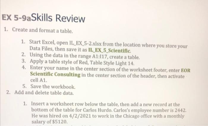
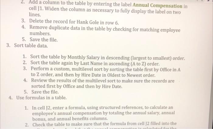
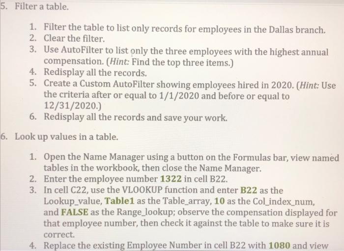
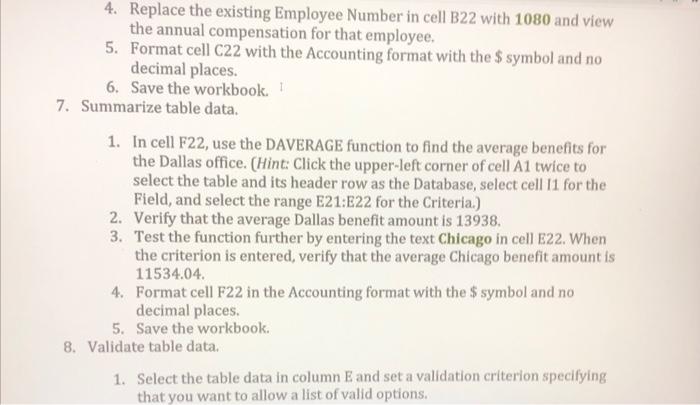
1. Create and format a table. 1. Start Excel, open IL_EX_5-2.xlsx from the location where you store your Data Files, then save it as IL_EX_5_Scientific. 2. Using the data in the range A1:I17, create a table. 3. Apply a table style of Red, Table Style Light 14. 4. Enter your name in the center section of the worksheet footer, enter EOR Scientific Consulting in the center section of the header, then activate cell A1. 5. Save the workbook. 2. Add and delete table data. 1. Insert a worksheet row below the table, then add a new record at the bottom of the table for Carlos Hurdo. Carlos's employee number is 2442. He was hired on 4/2/2021 to work in the Chicago office with a monthly salary of $5120. 2. Add a column to the table by entering the label Annual Compensation in cell J1. Widen the column as necessary to fully display the label on two lines. 3. Delete the record for Hank Gole in row 6. 4. Remove duplicate data in the table by checking for matching employee numbers. 5. Save the file. 3. Sort table data. 1. Sort the table by Monthly Salary in descending (largest to smallest) order. 2. Sort the table again by Last Name in ascending (A to Z) order. 3. Perform a custom, multilevel sort by sorting the table first by Office in A to Z order, and then by Hire Date in Oldest to Newest order. 4. Review the results of the multilevel sort to make sure the records are sorted first by Office and then by Hire Date. 5. Save the file. 4. Use formulas in a table. 1. In cell J2, enter a formula, using structured references, to calculate an employee's annual compensation by totaling the annual salary, annual bonus, and annual benefits columns. 2. Check the table to make sure that the formula from cell J2 filled into the cells in column J, and that the annual compensation is calculated for the cells in the column. 3. Add a total row to display the total annual compensation for all employees. 4. Change the function in the total row to display the average annual compensation. Change the label in cell A17 from Total to Average. 5. Save your work. 5. Filter a table. 1. Filter the table to list only records for employees in the Dallas branch. 1. Filter the table to list only records for employees in the Dallas branch. 2. Clear the filter. 3. Use AutoFilter to list pnly the three employees with the highest annual compensation. (Hint: Find the top three items.) 4. Redisplay all the records. 5. Create a Custom AutoFilter showing employees hired in 2020. (Hint: Use the criteria after or equal to 1/1/2020 and before or equal to 12/31/2020.) 6. Redisplay all the records and save your work. 6. Look up values in a table. 1. Open the Name Manager using a button on the Formulas bar, view named tables in the workbook, then close the Name Manager. 2. Enter the employee number 1322 in cell B22. 3. In cell C22, use the VLOOKUP function and enter B22 as the Lookup_value, Table1 as the Table_array, 10 as the Col_index_num, and FALSE as the Range_lookup; observe the compensation displayed for that employee number, then check it against the table to make sure it is correct. 4. Replace the existing Employee Number in cell B22 with 1080 and view 4. Replace the existing Employee Number in cell B22 with 1080 and view the annual compensation for that employee. 5. Format cell C22 with the Accounting format with the $ symbol and no decimal places. 6. Save the workbook. 7. Summarize table data. 1. In cell F22, use the DAVERAGE function to find the average benefits for the Dallas office. (Hint: Click the upper-left corner of cell A1 twice to select the table and its header row as the Database, select cell II for the Field, and select the range E21:E22 for the Criteria.) 2. Verify that the average Dallas benefit amount is 13938. 3. Test the function further by entering the text Chicago in cell E22. When the criterion is entered, verify that the average Chicago benefit amount is 11534.04. 4. Format cell F22 in the Accounting format with the $ symbol and no decimal places. 5. Save the workbook. 8. Validate table data. 1. Select the table data in column E and set a validation criterion specifying that you want to allow a list of valid options. 1. Select the table data in column E and set a validation criterion specifying that you want to allow a list of valid options. 2. Enter a list of valid options that restricts the entries to LA, Chicago, and Dallas. Remember to use a comma between each item in the list. 3. Confirm that the options will appear in an in-cell dropdown list, then close the dialog box. 4. Add a row to the bottom of the table. Select cell E17, open the dropdown list, then click Chicago. 5. Complete the new record by adding an Employee Number of 1119, a First Name of Cate, a Last Name of Smith, a Hire Date of 10/1/2021, and a monthly salary of $5000. Compare your screen to Figure 5-21
