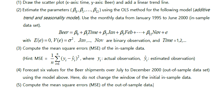
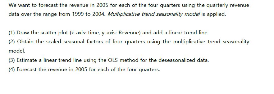
(1) Draw the scatter plot (x-axis: time, y-axis: Beer) and add a linear trend line. (2) Estimate the parameters ( Po, P,,...; 12 ) using the OLS method for the following model (additive trend and seasonality model). Use the monthly data from January 1995 to June 2000 (in-sample data set). Beer = Bo + B.Time + B, Jan+ B Feb + . . .+ BizNovte with E(e) =0, V(e) =o' . Jan.., Nov are binary observation, and Time = 1,2,. (3) Compute the mean square errors (MSE) of the in-sample data. n (Hint: MSE = -> (y, -y;)' , where y,: actual observation, );: estimated observation) n i=1 (4) Forecast six values for the Beer shipments over July to December 2000 (out-of-sample data set) using the model above. Here, do not change the window of the initial in-sample data. (5) Compute the mean square errors (MSE) of the out-of-sample data.|We want to forecast the revenue in 2005 for each of the four quarters using the quarterly revenue data over the range from 1999 to 2004. Mufhffc'arfve trend seasonafr'g/ mode; is applied. (1] Draw the scatter plot {mtaxis: time, yaxis: Revenue} and add a linear trend line. (2] Obtain the scaled seasonal factors of four quarters using the multiplicative trend seasonality model. (3] Estimate a linear trend line using the OLE method for the deseasonalized data. (4] Forecast the revenue in 2005 for each of the four quarters