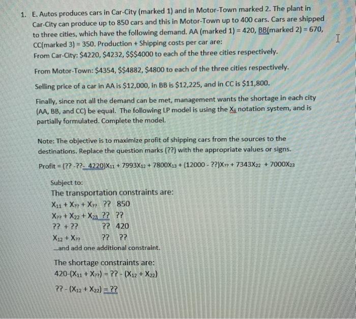
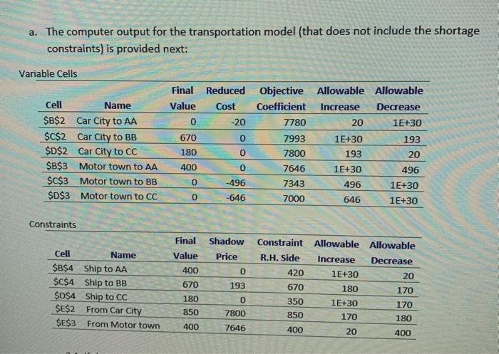
1. E. Autos produces cars in Car-City (marked 1) and in Motor-Town marked 2. The plant in Car-City can produce up to 850 cars and this in Motor-Town up to 400 cars. Cars are shipped to three cities, which have the following demand. AA (marked 1) = 420, BB(marked 2) = 670, CC(marked 3) = 350. Production + Shipping costs per car are: %3D From Car-City: $4220, $4232, $$$4000 to each of the three cities respectively. From Motor-Town: $4354, $$4882, $4800 to each of the three cities respectively. Selling price of a car in AA is $12,000, in BB is $12,225, and in CC is $11,800. Finally, since not all the demand can be met, management wants the shortage in each city (AA, BB, and CC) be equal. The following LP model is using the X notation system, and is partially formulated. Complete the model. Note: The objective is to maximize profit of shipping cars from the sources to the destinations. Replace the question marks (??) with the appropriate values or signs. Profit = (?? -??- 4220)X11 + 7993X12 + 7800X13 + (12000 - ??)X7 + 7343X22 + 7000X23 Subject to: The transportation constraints are: X11 + X + Xm ?? 850 Xp+ X22 + X23 ?? ?? ?? +?? ?? 420 X12 + X7 ?? ?? ..and add one additional constraint. The shortage constraints are: 420-(X11 + X) = ?? - (X12 + X22) ?? - (X12 + X22) = ?? a. The computer output for the transportation model (that does not include the shortage constraints) is provided next: Variable Cells Final Reduced Objective Allowable Allowable Cell Name Value Cost Coefficient Increase Decrease $B$2 Car City to AA -20 7780 20 1E+30 $C$2 Car City to BB 670 0. 7993 1E+30 193 $D$2 Car City to CC 180 7800 193 20 B$3 Motor town to AA 400 7646 1E+30 496 $C$3 Motor town to BB 0. -496 7343 496 1E+30 $D$3 Motor town to CC 0. -646 7000 646 1E+30 Constraints Final Shadow Constraint Allowable Allowable Cell Name Value Price R.H. Side Increase Decrease $B$4 Ship to AA $C$4 Ship to BB $D$4 Ship to CC SE$2 From Car City 400 0. 420 1E+30 20 670 193 670 180 170 180 0. 350 1E+30 170 850 7800 850 170 180 SE$3 From Motor town 400 7646 400 20 400