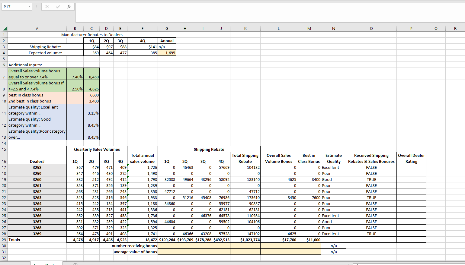
1. In column P, Ken wants to see an overall effectiveness rating of all of their dealers. All of the dealers should be classified as either Excellent, Good or Poor based upon the following criteria:

Excellent: Received a Quarterly Shipping Rebate (completed in step 4) in 3 or more of the 4 quarters AND also reached their Overall Sales Volume Bonus.

Good: Received a Quarterly Shipping Rebate (completed in step 4) in at least 1 of the 4 quarters OR also reached their Overall Sales Volume Bonus.

Poor: They were neither Excellent nor Good.

2. Create Conditional Formatting Rules to change the formatting on cells in column P.Create a rule to change the formatting on cells equal to "Excellent" to Green Fill with Dark Green Text formatting.

Create a rule to change the formatting on cells equal to "Good" to display Yellow Fill with Dark Yellow Text formatting.

Create a rule to change the formatting on cells equal to "Poor" to display Light Red Fill with Dark Red Text formatting. Hint: These 3 different formats are 3 the top 3 choices of conditional formatting so use the values from this dropdown as opposed to making up your own coloring scheme. It should look something like the accompanying image when complete (but with different values in the different cells).

3. In rows 30 & 31 for each column that contains a rebate/bonus (G through M), create formulas that determine the number of dealerships receiving the bonus and the average value of the bonus:In cells G30:M30 determine the number (count) of dealerships receiving this rebate/bonus.

In cells G31:M31 determine the average value of the bonus (include dealerships that did not earn a bonus in the average calculation). Apply Currency number formatting to the values.

4.

In cells B17:E28, Ken wants the dealerships quarterly cells that are Greater Than or Equal to (>=) the quarterly expected volume cells (C4:F4) to be formatted with White, Background 1 font color and Green fill (6th color from the left). You must create a Conditional Formatting rule using a formula to accomplish this.In cell B17 create a conditional formatting rule that uses a formula to determine whether or not to format the cell in with White, Background 1 font color and Green fill (6^th color from the left on the Fill tab). Use a mixed reference making the row absolute to the quarterly expected volume cell for that quarter.

Use the format painter to copy the conditional formatting across and down throughout cells B17:E28

PLEASE MAKE FORMULAS AND PROVIDE EXPLANATIONS TO THE QUESTIONS ABOVE I NEED TO LEARN HOW TO DO IT AND IM SO LOST

pir x