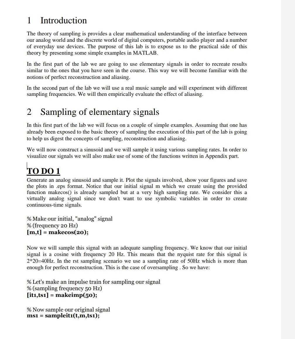
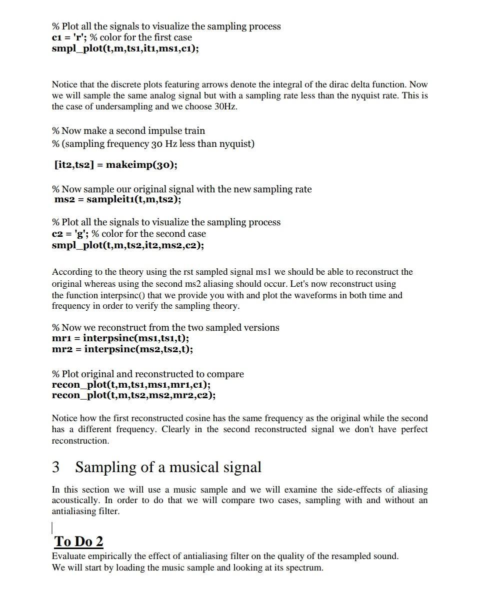
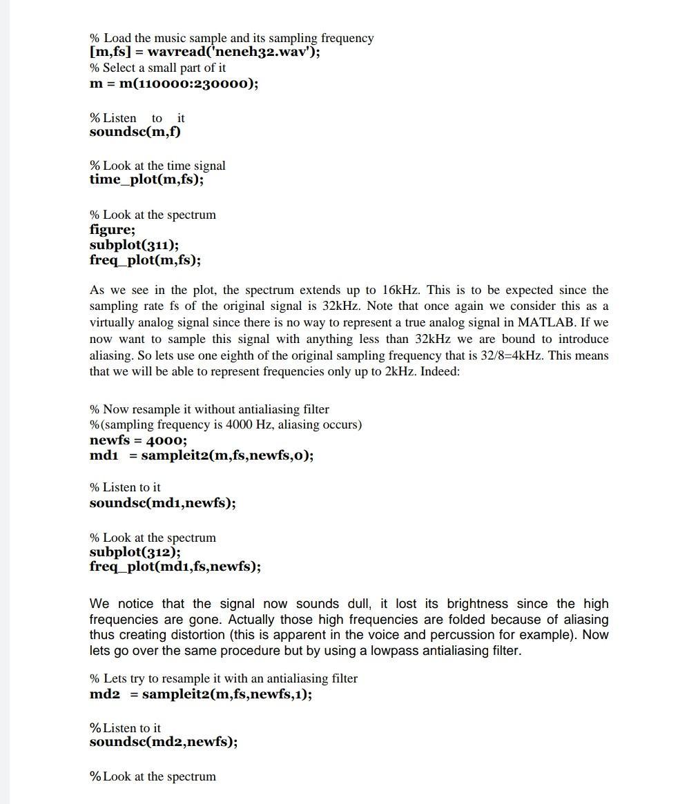
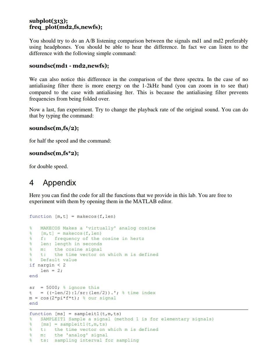1 Introduction The theory of sampling is provides a clear mathematical understanding of the interface between our analog world and the discrete world of digital computers, portable audio player and a number of everyday use devices. The purpose of this lab is to expose us to the practical side of this theory by presenting some simple examples in MATLAB. In the first part of the lab we are going to use elementary signals in order to recreate results similar to the ones that you have seen in the course. This way we will become familiar with the notions of perfect reconstruction and aliasing. In the second part of the lab we will use a real music sample and will experiment with different sampling frequencies. We will then empirically evaluate the effect of aliasing. 2 Sampling of elementary signals In this first part of the lab we will focus on a couple of simple examples. Assuming that one has already been exposed to the basic theory of sampling the execution of this part of the lab is going to help us digest the concepts of sampling, reconstruction and aliasing. We will now construct a sinusoid and we will sample it using various sampling rates. In order to visualize our signals we will also make use of some of the functions written in Appendix part. TO DO 1 Generate an analog sinusoid and sample it. Plot the signals involved, show your figures and save the plots in .eps format. Notice that our initial signal m which we create using the provided function makecos() is already sampled but at a very high sampling rate. We consider this a virtually analog signal since we don't want to use symbolic variables in order to create continuous-time signals. % Make our initial, "analog" signal % (frequency 20 Hz) [m,t] = makecos(20); Now we will sample this signal with an adequate sampling frequency. We know that our initial signal is a cosine with frequency 20 Hz. This means that the nyquist rate for this signal is 2*20=40Hz. In the rst sampling scenario we use a sampling rate of 50Hz which is more than enough for perfect reconstruction. This is the case of oversampling . So we have: % Let's make an impulse train for sampling our signal % (sampling frequency 50 Hz) [it1,ts1] = makeimp(50); % Now sample our original signal ms1 = sampleit1(t,m,ts1); % Plot all the signals to visualize the sampling process c1 = 'r'; % color for the first case smpl_plot(t,m,ts1,it1,ms1,c1); Notice that the discrete plots featuring arrows denote the integral of the dirac delta function. Now we will sample the same analog signal but with a sampling rate less than the nyquist rate. This is the case of undersampling and we choose 30Hz. % Now make a second impulse train % (sampling frequency 30 Hz less than nyquist) [it2,ts2] = makeimp(30); % Now sample our original signal with the new sampling rate ms2 = sampleit1(t,m,ts2); % Plot all the signals to visualize the sampling process c2 = 'g'; % color for the second case smpl_plot(t,m,ts2,it2,ms2,c2); According to the theory using the rst sampled signal ms1 we should be able to reconstruct the original whereas using the second ms2 aliasing should occur. Let's now reconstruct using the function interpsinc() that we provide you with and plot the waveforms in both time and frequency in order to verify the sampling theory. % Now we reconstruct from the two sampled versions mr1 = interpsinc(ms1,ts1,t); mr2 = interpsinc(ms2,ts2,t); % Plot original and reconstructed to compare recon_plot(t,m,ts1,ms1,mr1,c1); recon_plot(t,m,ts2,ms2,mr2,c2); Notice how the first reconstructed cosine has the same frequency as the original while the second has a different frequency. Clearly in the second reconstructed signal we don't have perfect reconstruction. 3 Sampling of a musical signal In this section we will use a music sample and we will examine the side-effects of aliasing acoustically. In order to do that we will compare two cases, sampling with and without an antialiasing filter. To Do 2 Evaluate empirically the effect of antialiasing filter on the quality of the resampled sound. We will start by loading the music sample and looking at its spectrum. % Load the music sample and its sampling frequency [m,fs] = wavread('neneh32.wav'); % Select a small part of it m = m(110000:230000); % Listen to it soundsc(m,f) % Look at the time signal time_plot(m,fs); % Look at the spectrum figure; subplot(311); freq_plot(m,fs); As we see in the plot, the spectrum extends up to 16kHz. This is to be expected since the sampling rate fs of the original signal is 32kHz. Note that once again we consider this as a virtually analog signal since there is no way to represent a true analog signal in MATLAB. If we now want to sample this signal with anything less than 32kHz we are bound to introduce aliasing. So lets use one eighth of the original sampling frequency that is 32/8=4kHz. This means that we will be able to represent frequencies only up to 2kHz. Indeed: % Now resample it without antialiasing filter %(sampling frequency is 4000 Hz, aliasing occurs) newfs = 4000; md1 = sampleit2(m,fs,newfs,0); % Listen to it soundsc(md1,newfs); % Look at the spectrum subplot(312); freq_plot(md1,fs,newfs); We notice that the signal now sounds dull, it lost its brightness since the high frequencies are gone. Actually those high frequencies are folded because of aliasing thus creating distortion (this is apparent in the voice and percussion for example). Now lets go over the same procedure but by using a lowpass antialiasing filter. % Lets try to resample it with an antialiasing filter md2 = sampleit2(m,fs,newfs,1); %Listen to it soundsc(md2,newfs); %Look at the spectrum subplot(313); freq_plot(md2,fs,newfs); You should try to do an A/B listening comparison between the signals md1 and md2 preferably using headphones. You should be able to hear the difference. In fact we can listen to the difference with the following simple command: soundsc(md1 - md2,newfs); We can also notice this difference in the comparison of the three spectra. In the case of no antialiasing filter there is more energy on the 1-2kHz band (you can zoom in to see that) compared to the case with antialiasing lter. This is because the antialiasing filter prevents frequencies from being folded over. Now a last, fun experiment. Try to change the playback rate of the original sound. You can do that by typing the command: soundsc(m,fs/2); for half the speed and the command: soundsc(m,fs*2); for double speed. 4 Appendix Here you can find the code for all the functions that we provide in this lab. You are free to experiment with them by opening them in the MATLAB editor. function [m,t] = makecos(f,len) % MAKECOS Makes a 'virtually' analog cosine % [m,t] = makecos(f,len) % f: frequency of the cosine in hertz % len: length in seconds % m: the cosine signal % t: the time vector on which m is defined % Default value if nargin =0); stem(ts(idx),ms(idx),'fill',[c,'^']); hold on; idx = find(ms= 0); stem(ts(idx),ms(idx),'fill',[c,'^']); hold on; idx = find(ms 1 Introduction The theory of sampling is provides a clear mathematical understanding of the interface between our analog world and the discrete world of digital computers, portable audio player and a number of everyday use devices. The purpose of this lab is to expose us to the practical side of this theory by presenting some simple examples in MATLAB. In the first part of the lab we are going to use elementary signals in order to recreate results similar to the ones that you have seen in the course. This way we will become familiar with the notions of perfect reconstruction and aliasing. In the second part of the lab we will use a real music sample and will experiment with different sampling frequencies. We will then empirically evaluate the effect of aliasing. 2 Sampling of elementary signals In this first part of the lab we will focus on a couple of simple examples. Assuming that one has already been exposed to the basic theory of sampling the execution of this part of the lab is going to help us digest the concepts of sampling, reconstruction and aliasing. We will now construct a sinusoid and we will sample it using various sampling rates. In order to visualize our signals we will also make use of some of the functions written in Appendix part. TO DO 1 Generate an analog sinusoid and sample it. Plot the signals involved, show your figures and save the plots in .eps format. Notice that our initial signal m which we create using the provided function makecos() is already sampled but at a very high sampling rate. We consider this a virtually analog signal since we don't want to use symbolic variables in order to create continuous-time signals. % Make our initial, "analog" signal % (frequency 20 Hz) [m,t] = makecos(20); Now we will sample this signal with an adequate sampling frequency. We know that our initial signal is a cosine with frequency 20 Hz. This means that the nyquist rate for this signal is 2*20=40Hz. In the rst sampling scenario we use a sampling rate of 50Hz which is more than enough for perfect reconstruction. This is the case of oversampling. So we have: % Let's make an impulse train for sampling our signal % (sampling frequency 50 Hz) [it1, ts1] = makeimp(50); % Now sample our original signal ms1 = sampleiti(t,m,ts1); % Plot all the signals to visualize the sampling process c1 = 'r'; % color for the first case smpl_plot(t,m,ts, iti,ms1,c1); Notice that the discrete plots featuring arrows denote the integral of the dirac delta function. Now we will sample the same analog signal but with a sampling rate less than the nyquist rate. This is the case of undersampling and we choose 30Hz. % Now make a second impulse train % (sampling frequency 30 Hz less than nyquist) [it2, ts2] = makeimp(30); % Now sample our original signal with the new sampling rate ms2 = sampleitit,m,ts2); % Plot all the signals to visualize the sampling process c2 = 'g'; % color for the second case smpl_plot(t,m,ts2,it2, ms2,c2); According to the theory using the rst sampled signal msl we should be able to reconstruct the original whereas using the second ms2 aliasing should occur. Let's now reconstruct using the function interpsinc() that we provide you with and plot the waveforms in both time and frequency in order to verify the sampling theory. % Now we reconstruct from the two sampled versions mri = interpsinc(msi, ts1,t); mr2 = interpsinc(ms2, ts2,t); % Plot original and reconstructed to compare recon_plot(t,m,ts1,ms1,mri,c1); recon_plot(t,m,ts2,ms2,mr2,c2); Notice how the first reconstructed cosine has the same frequency as the original while the second has a different frequency. Clearly in the second reconstructed signal we don't have perfect reconstruction. 3 Sampling of a musical signal In this section we will use a music sample and we will examine the side-effects of aliasing acoustically. In order to do that we will compare two cases, sampling with and without an antialiasing filter. To Do 2 Evaluate empirically the effect of antialiasing filter on the quality of the resampled sound. We will start by loading the music sample and looking at its spectrum. % Load the music sample and its sampling frequency [m,fs] = wavread('neneh32.wav"); % Select a small part of it m = m(110000:230000); % Listen to it soundsc(m,f) % Look at the time signal time_plot(m,fs); % Look at the spectrum figure; subplot(311); freq_plot(m,fs); As we see in the plot, the spectrum extends up to 16kHz. This is to be expected since the sampling rate fs of the original signal is 32kHz. Note that once again we consider this as a virtually analog signal since there is no way to represent a true analog signal in MATLAB. If we now want to sample this signal with anything less than 32kHz we are bound to introduce aliasing. So lets use one eighth of the original sampling frequency that is 32/8=4kHz. This means that we will be able to represent frequencies only up to 2kHz. Indeed: % Now resample it without antialiasing filter %(sampling frequency is 4000 Hz, aliasing occurs) newfs = 4000; md = sampleit (m,fs,newfs,o); % Listen to it soundsc(md,newfs); % Look at the spectrum subplot(312); freq_plot(md, fs,newfs); We notice that signal now sounds ull, it lost its brightness since the high frequencies are gone. Actually those high frequencies are folded because of aliasing thus creating distortion (this is apparent in the voice and percussion for example). Now lets go over the same procedure but by using a lowpass antialiasing filter. % Lets try to resample it with an antialiasing filter md2 = sampleit2(m,fs,newfs,1); % Listen to it soundsc(md2, newfs); % Look at the spectrum subplot(313); freq_plot(md2,fs,newfs); You should try to do an A/B listening comparison between the signals mdl and md2 preferably using headphones. You should be able to hear the difference. In fact we can listen to the difference with the following simple command: soundsc(md - md2,newfs); We can also notice this difference in the comparison of the three spectra. In the case of no antialiasing filter there is more energy on the 1-2kHz band (you can zoom in to see that) compared to the case with antialiasing Iter. This is because the antialiasing filter prevents frequencies from being folded over. Now a last, fun experiment. Try to change the playback rate of the original sound. You can do that by typing the command: soundsc(m,fs/2); for half the speed and the command: soundsc(m,fs*2); for double speed. 4 Appendix Here you can find the code for all the functions that we provide in this lab. You are free to experiment with them by opening them in the MATLAB editor. function [m, t] = makecos(f, len) MAKECOS Makes a 'virtually' analog cosine [m, t] = makecos(f, len) g f: frequency of the cosine in hertz 3 len: length in seconds m: the cosine signal 8 the time vector on which mis defined Default value if nargin