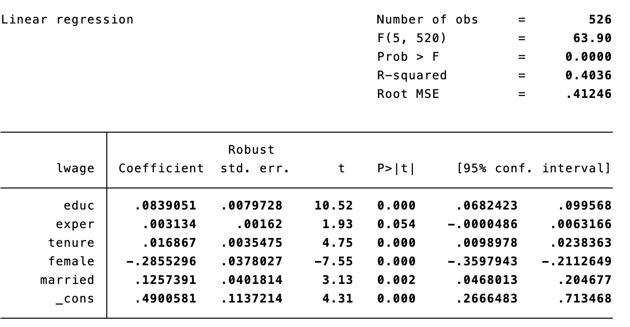
1. Is there a gender wage gap in the data (interpret)? Is it statistically significant?

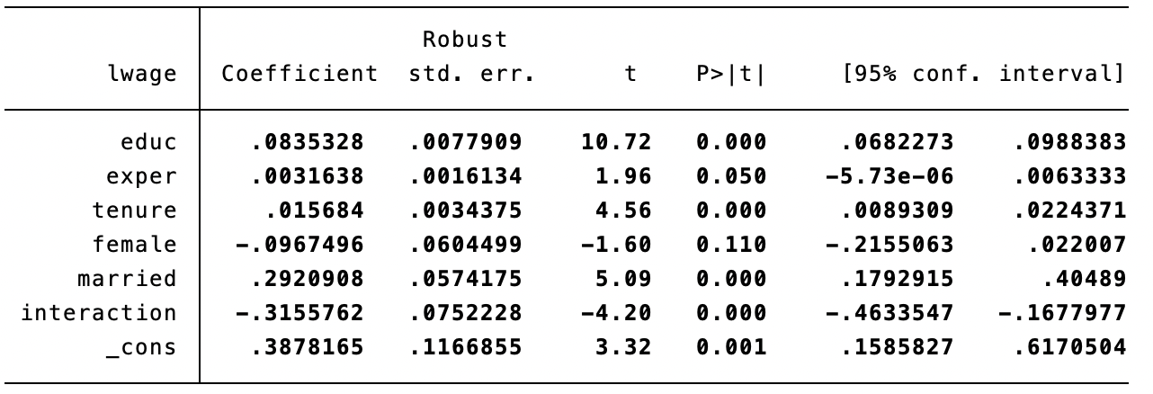
2. Add an interaction term involving female and married to the model and report the SRF

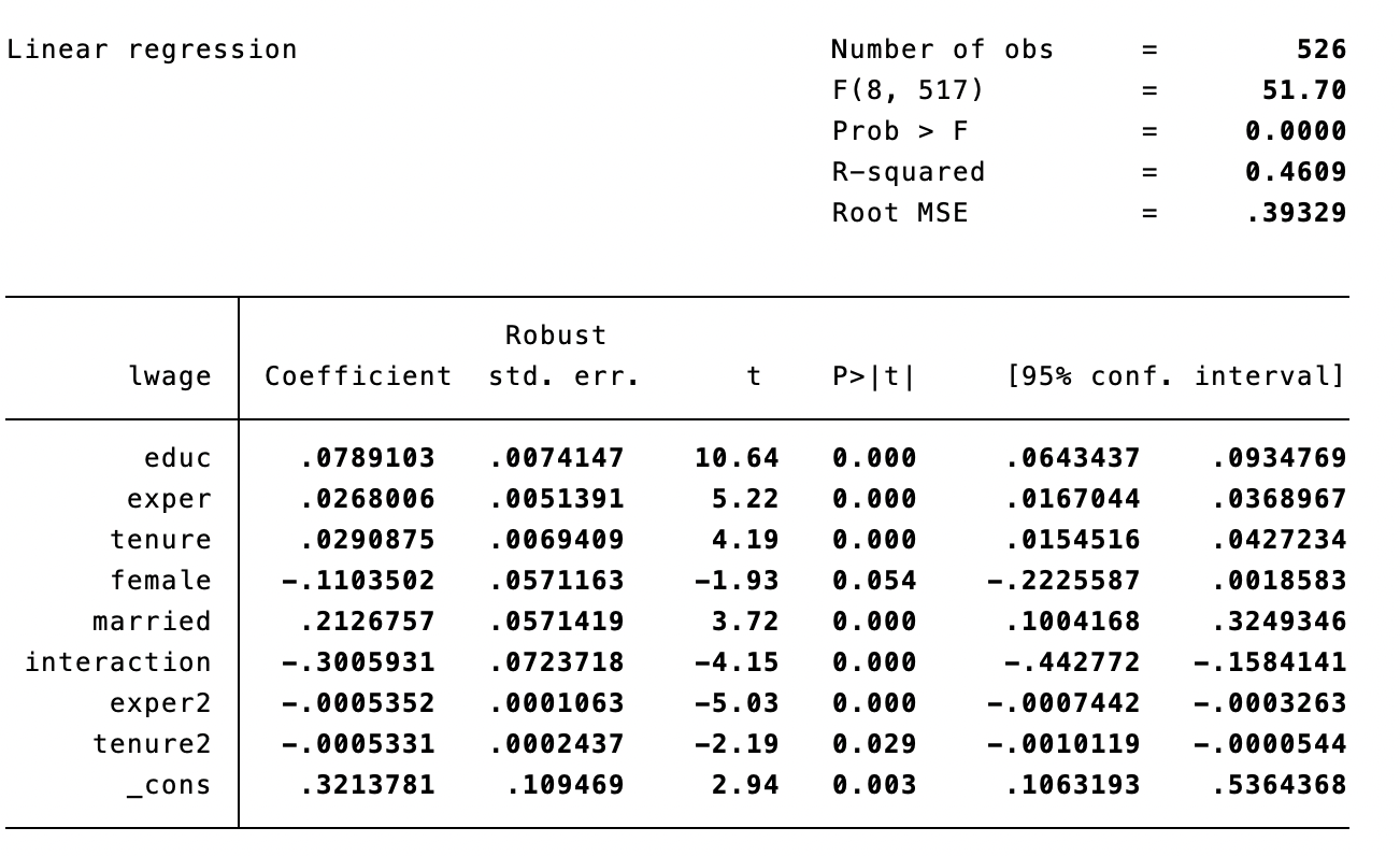
3. Interpret the coefficient of the interaction term. 4. Add exper² and tenure² to the model and report the SRF.5. What is the effect of one additional year of experience on wage for someone with only 1 year of experience? What about for someone with 15 years of experience?

6. Someone argues that the effect of one more year of education on wage is different across gender. Modify your model to test this argument. Report the SRF. Construct a 95% confidence interval for the coefficient of the variable that captures the effect.

The data file 'wage' contains the following data: 1. wage 2. educ 3. exper 4. tenure 6. female 7. married average hourly earnings in $ years of education years potential experience years with current employer =1 if female =1 if married Linear regression 526 F(5, = 63.90 Number of obs 520) Prob > F R-squared Root MSE II II 11 = = 0.0000 0.4036 .41246 II = Robust std. err. lwage Coefficient t P> [t| [95% conf. interval] educ .0079728 .00162 10.52 1.93 0.000 0.054 .0682423 -.0000486 .0035475 exper tenure female married .0839051 .003134 .016867 -.2855296 .1257391 .4900581 4.75 -7.55 3.13 .0378 027 0.000 0.000 0.002 .099568 .0063166 .0238363 -.2112649 .204677 .0098978 -.3597943 .0468013 .2666483 .0401814 _cons . 1137214 4.31 0.000 .713468 Robust lwage Coefficient std. err. t P> [t| [95% conf. interval] educ .0835328 0.000 0682273 .0031638 0.050 exper tenure female 10.72 1.96 4.56 -1.60 .015684 .0077909 .0016134 .0034375 .0604499 .0574175 .0752228 .1166855 0.000 0.110 -5.73e-06 .0089309 -. 2155063 . 1792915 .0967496 0988383 .0063333 .0224371 022007 .40489 -.1677977 .6170504 5.09 0.000 married interaction .2920908 -.3155762 -.4633547 -4.20 3.32 0.000 0.001 _cons .3878165 . 1585827 Linear regression = Number of obs F(8, 517) Prob > F R-squared Root MSE 526 51.70 0.0000 = = 0.4609 = 39329 Robust lwage Coefficient std. err. t P>|t| [95% conf. interval] educ .0789103 .0074147 0.000 . 10.64 5.22 .0268006 0.000 0934769 .0368967 0427234 .0051391 .0069409 .0571163 .0290875 4.19 -1.93 0.000 0.054 .1103502 0018583 exper tenure female married interaction exper2 tenure2 .2126757 3.72 .0571419 .0723718 3249346 .0643437 .0167044 .0154516 -.2225587 . 1004168 -.442772 -.0007442 -.0010119 1063193 -.3005931 -.0005352 -.0005331 0.000 0.000 0.000 0.029 -4.15 -5.03 -2.19 .0001063 0002437 . 109469 -.1584141 -.0003263 -.0000544 _cons 3213781 2.94 0.003 5364368 The data file 'wage' contains the following data: 1. wage 2. educ 3. exper 4. tenure 6. female 7. married average hourly earnings in $ years of education years potential experience years with current employer =1 if female =1 if married Linear regression 526 F(5, = 63.90 Number of obs 520) Prob > F R-squared Root MSE II II 11 = = 0.0000 0.4036 .41246 II = Robust std. err. lwage Coefficient t P> [t| [95% conf. interval] educ .0079728 .00162 10.52 1.93 0.000 0.054 .0682423 -.0000486 .0035475 exper tenure female married .0839051 .003134 .016867 -.2855296 .1257391 .4900581 4.75 -7.55 3.13 .0378 027 0.000 0.000 0.002 .099568 .0063166 .0238363 -.2112649 .204677 .0098978 -.3597943 .0468013 .2666483 .0401814 _cons . 1137214 4.31 0.000 .713468 Robust lwage Coefficient std. err. t P> [t| [95% conf. interval] educ .0835328 0.000 0682273 .0031638 0.050 exper tenure female 10.72 1.96 4.56 -1.60 .015684 .0077909 .0016134 .0034375 .0604499 .0574175 .0752228 .1166855 0.000 0.110 -5.73e-06 .0089309 -. 2155063 . 1792915 .0967496 0988383 .0063333 .0224371 022007 .40489 -.1677977 .6170504 5.09 0.000 married interaction .2920908 -.3155762 -.4633547 -4.20 3.32 0.000 0.001 _cons .3878165 . 1585827 Linear regression = Number of obs F(8, 517) Prob > F R-squared Root MSE 526 51.70 0.0000 = = 0.4609 = 39329 Robust lwage Coefficient std. err. t P>|t| [95% conf. interval] educ .0789103 .0074147 0.000 . 10.64 5.22 .0268006 0.000 0934769 .0368967 0427234 .0051391 .0069409 .0571163 .0290875 4.19 -1.93 0.000 0.054 .1103502 0018583 exper tenure female married interaction exper2 tenure2 .2126757 3.72 .0571419 .0723718 3249346 .0643437 .0167044 .0154516 -.2225587 . 1004168 -.442772 -.0007442 -.0010119 1063193 -.3005931 -.0005352 -.0005331 0.000 0.000 0.000 0.029 -4.15 -5.03 -2.19 .0001063 0002437 . 109469 -.1584141 -.0003263 -.0000544 _cons 3213781 2.94 0.003 5364368