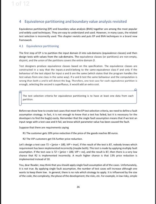
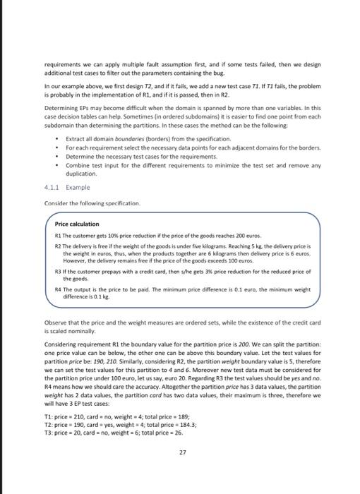
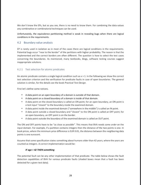
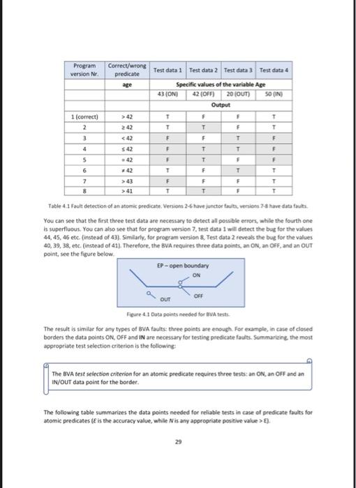
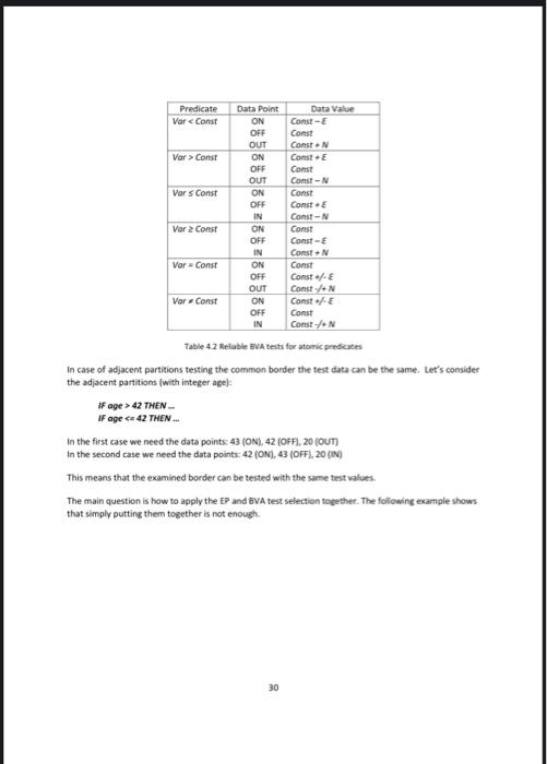
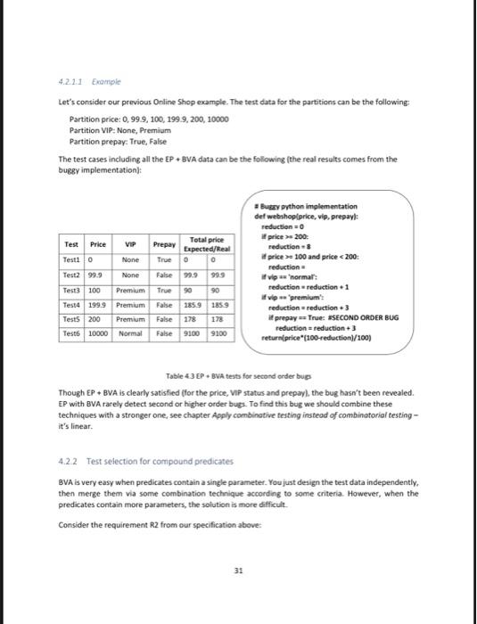
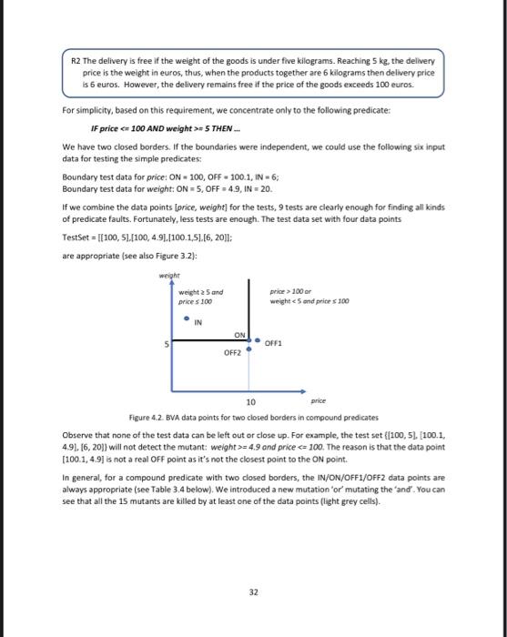
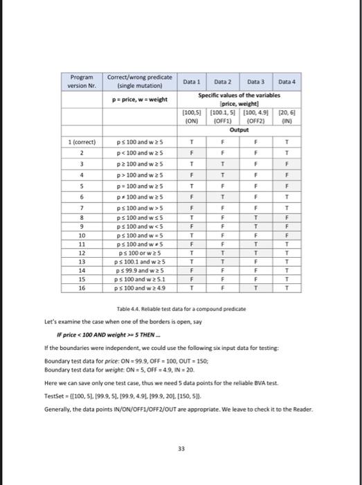
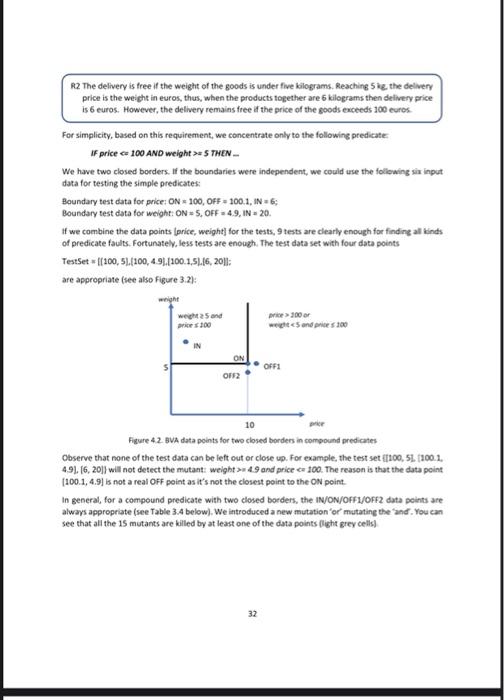
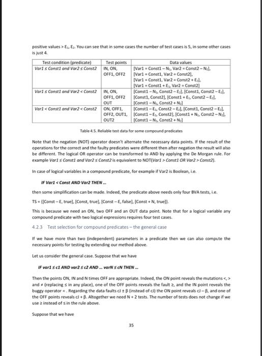
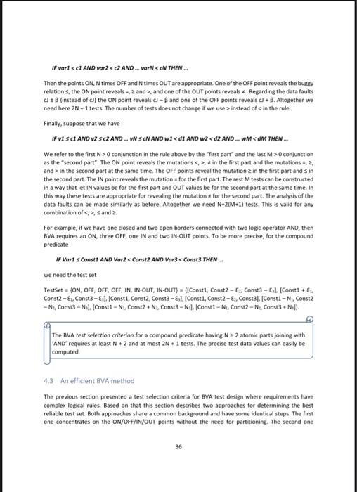
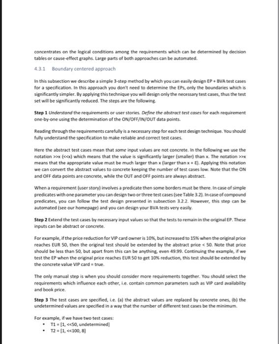
1 of 12 4 Equivalence partitioning and boundary value analysis revisited Equivalence partitioning (EP) and boundary value analysis (BVA) together are among the most popular and widely used techniques. They are easy to understand and used. However, in many cases, the related test selection is incorrectly used. This chapter revisits and puts EP and BVA techniques in a brand new framework 4.1 Equivalence partitioning The first step of EP is to partition the input domain D into sub-domains (equivalence classes) and then design tests with values from the sub-domains. The equivalence classes for partitions) are non-empty. disjoint, and the union of the partitions covers the entire domain D. Test designers produce equivalence dasses based on the specification. The equivalence classes are constructed in a way that the inputs a and belong to the same equivalence dass if and only if the behaviour of the test object for input and b are the same (which states that the program handles the test values from one class in the same way). If a and b test the same behaviour and the computation is wrong than both and will detect the bug. Therefore, one test case for each equivalence partition is enough, selecting the second is superfluous, it would add an extra cost. The test selection criteria for equivalence partitioning is to have at least one data from each partition Before we show how to create test cases that meet the EP test selection criteria, we need to define a fault assumption strategy. In fact, it is not enough to know that a test has failed, but it is necessary for the developers to find the bug(s) easily. Remember that the single fault assumption means that if we test an input range with a test case and it fail, we know which parameter value has been caused the fault. Suppose that there are requirements saying R1 The customer gets 10% price reduction if the price of the goods reaches 80 euros. R2 The VIP customers get 5% further price reduction. Let's design a test case TI - (price = 100, VIP true). If the result of the test is 87, nobody knows which requirement has been implemented incorrectly (maybe both). This test is made by applying multiply fault assumption. If the test case is T2 (price = 100, VIP = no), and the result is 87, then there is a very low chance that R2 is implemented incorrectly. A much higher chance is that 13% price reduction is implemented instead of 10 You, dear Reader, may think that you should apply single fault assumption all of the cases. Unfortunately, it is not true. By applying single fault assumption, the number of test cases will increase although one wants to keep them low. In general, there is no rule which strategy to apply. It is influenced by the size of the code, the complexity, the phase of the development, the risks, etc. For example, in low risky, simple 26 requirements we can apply multiple fault assumption first, and if some tests failed, then we design additional test cases to filter out the parameters containing the bug. In our example above, we first design 12, and if it fails, we add a new test case TI, If T1 fails, the problem is probably in the implementation of R1, and if it is passed, then in R2. Determining EPs may become difficult when the domain is spanned by more than one variables. In this case decision tables can help. Sometimes in ordered subdomains) is easier to find one point from each subdomain than determining the partitions. In these cases the method can be the following Extract all domain boundaries (borders) from the specification . For each requirement select the necessary data points for each adjacent domains for the borders. Determine the necessary test cases for the requirements Combine test input for the different requirements to minimize the test set and remove any duplication 4.1.1 Example Consider the following specification Price calculation R1 The customer gets 10% price reduction if the price of the goods reaches 200 euros R2 The delivery is free if the weight of the goods is under five kilograms. Reaching 5 kg the delivery price is the weight in euros, thus, when the products together are 6 kilograms then delivery price is 6 euros. However, the delivery remains free if the price of the goods exceeds 100 euros. R3 if the customer prepars with a credit card, then she gets 3x price reduction for the reduced price of the goods R4 The output is the price to be paid. The minimum price difference is 0.1 euro, the minimum weight difference is 0.1 kg Observe that the price and the weight measures are ordered sets, while the existence of the credit card is scaled nominally Considering requirement R1 the boundary value for the partition price is 200. We can split the partition: One price value can be below, the other one can be above this boundary value. Let the test values for partition price be: 190, 210. Similarly, considering R2, the partition weight boundary value is 5, therefore we can set the test values for this partition to 4 and 6. Moreover new test data must be considered for the partition price under 100 euro, let us say, euro 20. Regarding R3 the test values should be yes and no. R4 means how we should care the accuracy. Altogether the partition price has 3 data values, the partition weight has 2 data values, the partition cord has two data values, their maximum is three, therefore we will have 3 EP test cases: T1: price 210, card no, weight - 4; total price 189; T2. price 190, card yes, weight 4 total price - 184.3, 13: price = 20, card=no, weight = 6; total price = 26. 27 We don't know the EPs, but as you see, there is no need to know them. For combining the data values any combinative or combinatorial techniques can be used. Unfortunately, the equivalence partitioning method is weak in revealing bugs when there are logical conditions in the requirements. 4.2 Boundary value analysis EP is rarely used in isolation as in most of the cases there are logical conditions in the requirements. Potential bugs occur "near to the border of the partitions with higher probability. The reason is that the implemented and the correct borders are often different. The question is how to select the test cases concerning the boundaries. As mentioned, many textbooks, blogs, software testing courses suggest inappropriate solutions. 4.2.1 Test selection for atomic predicates An atomic predicate contains a single logical condition such as x > 1. In the following we show the correct test selection criterion and the verification for predicate faults in case of open boundaries. The general solution is similar, for the details see the book. Practical Test Design First let's define some notions. A data point on an open boundary of a domain is outside of that domain. A data point on a closed boundary of a domain is inside of that domain. A data point on the closed boundary is called an ON point: for an open boundary, an ON point is a test input "closest to the boundary inside the examined domain A data point inside the examined domain ("somewhere in the middle") is called an IN point A data point outside a closed boundary and "closest to the ON point is called an OFF point for an open boundary, an OFF point is on the border. A data point outside the boundary of the examined domain is called an OUT point. The ON and OFF points have to be as close as possible. This means that BVA needs some order on the input domain. For example, if a partition contains integers then the distance of the two points is one. In book prices, where the minimum price difference is EUR 0.01, the distance between the neighboring data points is one eurocent. Assume that some specification states something about humans older than 42 years, where the years are counted as integers. A correct implementation would be IF age > 42 THEN something The potential fault can be any other implementation of that predicate. The table below shows the fault detection capabilities of BVA for various predicate faults (shaded bones mean that a fault has been detected for a given test data) 28 Program version Nr. Correct/wrong predicate age Test data 1 Test data 2 Test data 3 Test data 4 Specific values of the variable Age 43 (ONI 42 (OFF) 20 (OUT) 50 N Output F T T T F T T F 1 (correct) 2 3 > 42 242 F F T F 43 >> 41 F 7 8 F F T T T F Table 4.1 Fault detection of an atomic predicate. Versions 2-6 have junctor tuits versions 18 have data faults. You can see that the first three test data are necessary to detect all possible errors, while the fourth one is superfluous. You can also see that for program version 7 test data 1 will detect the bug for the values 44, 45, 46 etc (instead of 43). Similarly, for program version & Test data 2 reveals the bug for the values 40,39, 38, etc. (instead of 41). Therefore, the BVA requires three data points, an ON, an OFF, and an OUT point, see the figure below. EP-open boundary ON OFF OUT Figure 41 Data points needed for VA tests The result is similar for any types of BVA faults: three points are enough. For example, in case of closed borders the data points ON, OFF and I are necessary for testing predicate faults. Summarizing the most appropriate test selection criterion is the following The BVA test selection criterion for an atomic predicate requires three tests: an ON, an OFF and an IN/OUT data point for the border. The following table summarizes the data points needed for reliable tests in case of predicate faults for atomic predicates (E is the accuracy value, while Nis any appropriate positive value>). 29 Predicate Vor Const Vor Const Data Point ON OFF OUT ON OFF OUT ON OFF IN ON OFF IN ON OFF OUT ON OFF IN Data Value Const-E Const Const. Const Const Const- Const Const. Cant- Const Const-E anst Const Const- ConstAN Const Const Const/N Var 2 Const Var - Const Vor Const Table 4.2 Reliable BVA tests for atomic predicates In case of adjacent partitions testing the common border the test data can be the same. Let's consider the adjacent partitions (with integer age IF age > 42 THEN IF age c42 THEN.. In the first case we need the data points: 43 (ON), 42 (OFF), 20 (OUT In the second case we need the data points: 42 (ON), 43 (OFF), 20 (1) This means that the examined border can be tested with the same test values The main question is how to apply the EP and BVA test selection together. The following example shows that simply putting them together is not enough 30 4.2.1.1 Example Let's consider our previous Online Shop example. The test data for the partitions can be the following: Partition price: 0,99.9, 100, 1999, 200, 10000 Partition VIP: None, Premium Partition prepay: True, False The test cases including all the EP + BVA data can be the following the real results comes from the buggy implementation) Test Prepay Total price Expected/Real 0 0 True Price VIP Test10 None Test2 99.9 None Test3 100 Premium Test4 199.9 Premium Tests 200 Premium Testo 10000 Normal False 99.9 99.9 True 90 90 False 1859 1859 False 178 178 False 9100 9100 Bugay python implementation de webshop price, vip, prepayl: reduction=0 price > 2003 reductions price > 100 and price = 5 THEN... We have two closed borders. If the boundaries were independent, we could use the following six input data for testing the simple predicates: Boundary test data for price: ON-100, OFF-100.1, IN - 6; Boundary test data for weight: ON = 5, OFF = 4.9, IN = 20. If we combine the data points [price, weight for the tests, 9 tests are clearly enough for finding all kinds of predicate faults. Fortunately, less tests are enough. The test data set with four data points TestSet = |(100, 51.[100, 4.91./100.1,5116, 2011: are appropriate (see also Figure 3.2): weight weight 25 and prices 100 price > 100 or weight = 4.9 and price 100 and w 25 p = 100 and w 25 p=100 and w25 ps 100 and 5 ps 100 and wss ps 100 and w c5 PS 100 and was ps 100 and we DS 100 or w25 ps 100.1 and w25 P 99.9 and w25 PS 100 and w 25.1 DS 100 and w 249 T F T 10 11 12 13 14 15 16 F T T F F T F F F F T T F F F T T F T T F F F T F F F T T T T T T Table 4.4. Reliable test data for a compound predicate Let's examine the case when one of the borders is open, say IF price =S THEN. of the boundaries were independent, we could use the following six input data for testing Boundary test data for price:ON - 99.9, OFF = 100, OUT = 150; Boundary test data for weight: ON = 5.OFF = 4.9 IN = 20 Here we can save only one test case, thus we need 5 data points for the reliable BVA test TestSet = {[100, 51, 199.9, 51. 19:9, 4.91, 199.9,201[150,51). Generally, the data points IN/ON/OFFI/OFF2/OUT are appropriate. We leave to check it to the Reader. 33 R2 The delivery is free if the weight of the goods is under five kilograms. Reaching 5 kg. the delivery price is the weight in euros, thus, when the products together are 6 kilograms the delivery price is 6 euros. However, the delivery remains free if the price of the goods exceeds 100 euros For simplicity, based on this requirement, we concentrate only to the following predicate: If price - 100 AND weight >=S THEN We have two closed borders. If the boundaries were independent, we could use the following six input data for testing the simple predicates Boundary test data for price: ON = 100, OFF = 100.1, IN = 6; Boundary test data for weight: ON = 5, OFF49, IN 20. If we combine the data points (price, weight for the tests, 9 tests are clearly enough for finding all kinds of predicate faults. Fortunately, less tests are enough. The test data set with four data points TestSet (100, 51.[100,4.9.200.1.516, 2011: are appropriate (see also Figure 3.2): whe weight and price 100 wc5 and 100 ON OF2 OFF1 10 Figure 42 BVA data points for two closed borders in compound predicates Observe that none of the test data can be left out or close up. For example, the test set 100,5L. (100.1. 4.91.16,20]) will not detect the mutant: weight > 4.9 and price e 100. The reason is that the data point (100.1, 4.9] is not a real OFF point as it's not the closest point to the ON point In general, for a compound predicate with two closed borders, the IN/ON/OFF1/OFF2 data points are always appropriate (see Table 3.4 below). We introduced a new mutation or mutating the and. You can see that all the 15 mutants are killed by at least one of the data points (light grey cells) 32 positive values > ELE). You can see that in some cases the number of test cases is 5, in some other cases is just 4 Test condition (predicate) Test points Data values Varls Const1 and Var2s Const2 IN ON, [Vari Const1 -- Ni. Var2 - Const2 - Nal. OFFI, OFF2 [Vari Const1, Var2 - Const2). Vari Const, Var2 Const2.. Var1 = Consti+Es Var2 = Const2] Varls Const1 and Var2 Consti or Ver2>Const2). In case of logical variables in a compound predicate, for example if var2 is Booleanie. IF Vari and replacings in any place), one of the OFF points reveals the fault 2, and the IN point reveals the buggy operator Regarding the data faults + Blinstead of ci) the ON point reveals cl-B, and one of the OFF points reveals cl B. Altogether we need N. 2 tests. The number of tests does not change if we use 2 instead of sin the rule above. Suppose that we have 35 If vari , and one of the OUT points reveals Regarding the data faults JJ: B (instead of c) the ON point reveals - and one of the OFF points reveals + B. Altogether we need here 2N + 1 tests. The number of tests does not change if we use instead of 0 conjunction in the rule above by the first part and the last M > O conjunction as the second part". The ON point reveals the mutations * in the first part and the mutations, 2, and > in the second part at the same time. The OFF points reveal the mutation 2 in the first part and sin the second part. The IN point reveals the mutation for the first part. The rest M tests can be constructed in a way that let IN values be for the first part and OUT values be for the second part at the same time. In this way these tests are appropriate for revealing the mutation for the second part. The analysis of the data faults can be made similarly as before. Altogether we need N+2[M+1) tests. This is valid for any combination of , Sand 2 For example, if we have one closed and two open borders connected with two logic operator AND, then BVA requires an ON, three OFF, one IN and two IN-OUT points. To be more precise, for the compound predicate If Varis Const1 AND Var2 > (>X means that the appropriate value must be much larger thanx (larger than x + . Applying this notation we can convert the abstract values to concrete keeping the number of test cases low. Note that the ON and OFF data points are concrete, while the OUT and OFF points are always abstract When a requirement (user story) involves a predicate then some borders must be there. In case of simple predicates with one parameter you can design two or three test cases (see Table 3.2). In case of compound predicates, you can follow the test design presented in subsection 3.2.2. However, this step can be automated (see our homepage) and you can design your BVA tests very easily Step 2 Extend the test cases by necessary input values so that the tests to remain in the original EP. These inputs can be abstract or concrete. For example, if the price reduction for VIP card owner is 10%, but increased to 15% when the original price reaches EUR 50, then the original test should be extended by the abstract price 1. In the following we show the correct test selection criterion and the verification for predicate faults in case of open boundaries. The general solution is similar, for the details see the book. Practical Test Design First let's define some notions. A data point on an open boundary of a domain is outside of that domain. A data point on a closed boundary of a domain is inside of that domain. A data point on the closed boundary is called an ON point: for an open boundary, an ON point is a test input "closest to the boundary inside the examined domain A data point inside the examined domain ("somewhere in the middle") is called an IN point A data point outside a closed boundary and "closest to the ON point is called an OFF point for an open boundary, an OFF point is on the border. A data point outside the boundary of the examined domain is called an OUT point. The ON and OFF points have to be as close as possible. This means that BVA needs some order on the input domain. For example, if a partition contains integers then the distance of the two points is one. In book prices, where the minimum price difference is EUR 0.01, the distance between the neighboring data points is one eurocent. Assume that some specification states something about humans older than 42 years, where the years are counted as integers. A correct implementation would be IF age > 42 THEN something The potential fault can be any other implementation of that predicate. The table below shows the fault detection capabilities of BVA for various predicate faults (shaded bones mean that a fault has been detected for a given test data) 28 Program version Nr. Correct/wrong predicate age Test data 1 Test data 2 Test data 3 Test data 4 Specific values of the variable Age 43 (ONI 42 (OFF) 20 (OUT) 50 N Output F T T T F T T F 1 (correct) 2 3 > 42 242 F F T F 43 >> 41 F 7 8 F F T T T F Table 4.1 Fault detection of an atomic predicate. Versions 2-6 have junctor tuits versions 18 have data faults. You can see that the first three test data are necessary to detect all possible errors, while the fourth one is superfluous. You can also see that for program version 7 test data 1 will detect the bug for the values 44, 45, 46 etc (instead of 43). Similarly, for program version & Test data 2 reveals the bug for the values 40,39, 38, etc. (instead of 41). Therefore, the BVA requires three data points, an ON, an OFF, and an OUT point, see the figure below. EP-open boundary ON OFF OUT Figure 41 Data points needed for VA tests The result is similar for any types of BVA faults: three points are enough. For example, in case of closed borders the data points ON, OFF and I are necessary for testing predicate faults. Summarizing the most appropriate test selection criterion is the following The BVA test selection criterion for an atomic predicate requires three tests: an ON, an OFF and an IN/OUT data point for the border. The following table summarizes the data points needed for reliable tests in case of predicate faults for atomic predicates (E is the accuracy value, while Nis any appropriate positive value>). 29 Predicate Vor Const Vor Const Data Point ON OFF OUT ON OFF OUT ON OFF IN ON OFF IN ON OFF OUT ON OFF IN Data Value Const-E Const Const. Const Const Const- Const Const. Cant- Const Const-E anst Const Const- ConstAN Const Const Const/N Var 2 Const Var - Const Vor Const Table 4.2 Reliable BVA tests for atomic predicates In case of adjacent partitions testing the common border the test data can be the same. Let's consider the adjacent partitions (with integer age IF age > 42 THEN IF age c42 THEN.. In the first case we need the data points: 43 (ON), 42 (OFF), 20 (OUT In the second case we need the data points: 42 (ON), 43 (OFF), 20 (1) This means that the examined border can be tested with the same test values The main question is how to apply the EP and BVA test selection together. The following example shows that simply putting them together is not enough 30 4.2.1.1 Example Let's consider our previous Online Shop example. The test data for the partitions can be the following: Partition price: 0,99.9, 100, 1999, 200, 10000 Partition VIP: None, Premium Partition prepay: True, False The test cases including all the EP + BVA data can be the following the real results comes from the buggy implementation) Test Prepay Total price Expected/Real 0 0 True Price VIP Test10 None Test2 99.9 None Test3 100 Premium Test4 199.9 Premium Tests 200 Premium Testo 10000 Normal False 99.9 99.9 True 90 90 False 1859 1859 False 178 178 False 9100 9100 Bugay python implementation de webshop price, vip, prepayl: reduction=0 price > 2003 reductions price > 100 and price = 5 THEN... We have two closed borders. If the boundaries were independent, we could use the following six input data for testing the simple predicates: Boundary test data for price: ON-100, OFF-100.1, IN - 6; Boundary test data for weight: ON = 5, OFF = 4.9, IN = 20. If we combine the data points [price, weight for the tests, 9 tests are clearly enough for finding all kinds of predicate faults. Fortunately, less tests are enough. The test data set with four data points TestSet = |(100, 51.[100, 4.91./100.1,5116, 2011: are appropriate (see also Figure 3.2): weight weight 25 and prices 100 price > 100 or weight = 4.9 and price 100 and w 25 p = 100 and w 25 p=100 and w25 ps 100 and 5 ps 100 and wss ps 100 and w c5 PS 100 and was ps 100 and we DS 100 or w25 ps 100.1 and w25 P 99.9 and w25 PS 100 and w 25.1 DS 100 and w 249 T F T 10 11 12 13 14 15 16 F T T F F T F F F F T T F F F T T F T T F F F T F F F T T T T T T Table 4.4. Reliable test data for a compound predicate Let's examine the case when one of the borders is open, say IF price =S THEN. of the boundaries were independent, we could use the following six input data for testing Boundary test data for price:ON - 99.9, OFF = 100, OUT = 150; Boundary test data for weight: ON = 5.OFF = 4.9 IN = 20 Here we can save only one test case, thus we need 5 data points for the reliable BVA test TestSet = {[100, 51, 199.9, 51. 19:9, 4.91, 199.9,201[150,51). Generally, the data points IN/ON/OFFI/OFF2/OUT are appropriate. We leave to check it to the Reader. 33 R2 The delivery is free if the weight of the goods is under five kilograms. Reaching 5 kg. the delivery price is the weight in euros, thus, when the products together are 6 kilograms the delivery price is 6 euros. However, the delivery remains free if the price of the goods exceeds 100 euros For simplicity, based on this requirement, we concentrate only to the following predicate: If price - 100 AND weight >=S THEN We have two closed borders. If the boundaries were independent, we could use the following six input data for testing the simple predicates Boundary test data for price: ON = 100, OFF = 100.1, IN = 6; Boundary test data for weight: ON = 5, OFF49, IN 20. If we combine the data points (price, weight for the tests, 9 tests are clearly enough for finding all kinds of predicate faults. Fortunately, less tests are enough. The test data set with four data points TestSet (100, 51.[100,4.9.200.1.516, 2011: are appropriate (see also Figure 3.2): whe weight and price 100 wc5 and 100 ON OF2 OFF1 10 Figure 42 BVA data points for two closed borders in compound predicates Observe that none of the test data can be left out or close up. For example, the test set 100,5L. (100.1. 4.91.16,20]) will not detect the mutant: weight > 4.9 and price e 100. The reason is that the data point (100.1, 4.9] is not a real OFF point as it's not the closest point to the ON point In general, for a compound predicate with two closed borders, the IN/ON/OFF1/OFF2 data points are always appropriate (see Table 3.4 below). We introduced a new mutation or mutating the and. You can see that all the 15 mutants are killed by at least one of the data points (light grey cells) 32 positive values > ELE). You can see that in some cases the number of test cases is 5, in some other cases is just 4 Test condition (predicate) Test points Data values Varls Const1 and Var2s Const2 IN ON, [Vari Const1 -- Ni. Var2 - Const2 - Nal. OFFI, OFF2 [Vari Const1, Var2 - Const2). Vari Const, Var2 Const2.. Var1 = Consti+Es Var2 = Const2] Varls Const1 and Var2 Consti or Ver2>Const2). In case of logical variables in a compound predicate, for example if var2 is Booleanie. IF Vari and replacings in any place), one of the OFF points reveals the fault 2, and the IN point reveals the buggy operator Regarding the data faults + Blinstead of ci) the ON point reveals cl-B, and one of the OFF points reveals cl B. Altogether we need N. 2 tests. The number of tests does not change if we use 2 instead of sin the rule above. Suppose that we have 35 If vari , and one of the OUT points reveals Regarding the data faults JJ: B (instead of c) the ON point reveals - and one of the OFF points reveals + B. Altogether we need here 2N + 1 tests. The number of tests does not change if we use instead of 0 conjunction in the rule above by the first part and the last M > O conjunction as the second part". The ON point reveals the mutations * in the first part and the mutations, 2, and > in the second part at the same time. The OFF points reveal the mutation 2 in the first part and sin the second part. The IN point reveals the mutation for the first part. The rest M tests can be constructed in a way that let IN values be for the first part and OUT values be for the second part at the same time. In this way these tests are appropriate for revealing the mutation for the second part. The analysis of the data faults can be made similarly as before. Altogether we need N+2[M+1) tests. This is valid for any combination of , Sand 2 For example, if we have one closed and two open borders connected with two logic operator AND, then BVA requires an ON, three OFF, one IN and two IN-OUT points. To be more precise, for the compound predicate If Varis Const1 AND Var2 > (>X means that the appropriate value must be much larger thanx (larger than x + . Applying this notation we can convert the abstract values to concrete keeping the number of test cases low. Note that the ON and OFF data points are concrete, while the OUT and OFF points are always abstract When a requirement (user story) involves a predicate then some borders must be there. In case of simple predicates with one parameter you can design two or three test cases (see Table 3.2). In case of compound predicates, you can follow the test design presented in subsection 3.2.2. However, this step can be automated (see our homepage) and you can design your BVA tests very easily Step 2 Extend the test cases by necessary input values so that the tests to remain in the original EP. These inputs can be abstract or concrete. For example, if the price reduction for VIP card owner is 10%, but increased to 15% when the original price reaches EUR 50, then the original test should be extended by the abstract price