1. The series begin with the first quarter of 2013 and end with the first quarter of 2018. Show the time plot series that display quarterly e-commerce retail sales as a percent of total U.S. retail sales. Show your plot in the space provided below: (2p.) 2. Calculate the moving averages for each observation in the data based on periods 1, 2, 3, and 4. Show the time plot of quarterly e-commerce retail sales along with the moving-average forecasts based on a span of k=4. Make sure to include the labels of x and y axes and adjust the values on the plot to show the possible changes more clearly over the time. Show your plot in the space provided below: (3p.) 3. Use the figure from question #2 to interpret the seasonal regularity to the time series data (e-commerce retail sales). For instance, in which quarters do you observe percent sales are the lowest or the highest, or in which quarters do you observe a rise or a decline? Compare and contrast the component that you observe in the time series and the moving averages. (4p.) 4. Calculate the centered moving average (CMA) and show the time plot of quarterly e-commerce retail sales along with the centered moving-average forecasts based on a span of k=4. Make sure to include the labels of x and y axes and adjust the values on the plot to show the possible changes more clearly over the time. In the space provided below, show your plot, and compare and interpret the trend of two series. (3p.) 5. Calculate the seasonal ratio of quarterly e-commerce retail sales and average these ratios by quarter. Show the resulting ratios based on the periods of 1, 2, 3 and 4 in the table below: Quarter Seasonality ratio 1 2 3 4 (4p.) 6. Regress the de-seasonality component of quarterly e-commerce retail sales on time component. In the space provided below, show your regression output and the regression equation using trend-and-season predictive model from the simple

Please use excel and show the process thankyou!

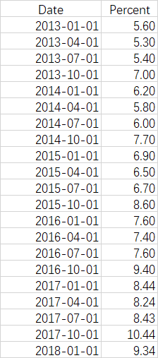
Date 2013-01-01 2013-04-01 2013-07-01 2013-10-01 2014-01-01 2014-04-01 2014-07-01 2014-10-01 2015-01-01 2015-04-01 2015-07-01 2015-10-01 2016-01-01 2016-04-01 2016-07-01 2016-10-01 2017-01-01 2017-04-01 2017-07-01 2017-10-01 2018-01-01 Percent 5.60 5.30 5.40 7.00 6.20 5.80 6.00 7.70 6.90 6.50 6.70 8.60 7.60 7.40 7.60 9.40 8.44 8.24 8.43 10.44 9.34 Date 2013-01-01 2013-04-01 2013-07-01 2013-10-01 2014-01-01 2014-04-01 2014-07-01 2014-10-01 2015-01-01 2015-04-01 2015-07-01 2015-10-01 2016-01-01 2016-04-01 2016-07-01 2016-10-01 2017-01-01 2017-04-01 2017-07-01 2017-10-01 2018-01-01 Percent 5.60 5.30 5.40 7.00 6.20 5.80 6.00 7.70 6.90 6.50 6.70 8.60 7.60 7.40 7.60 9.40 8.44 8.24 8.43 10.44 9.34