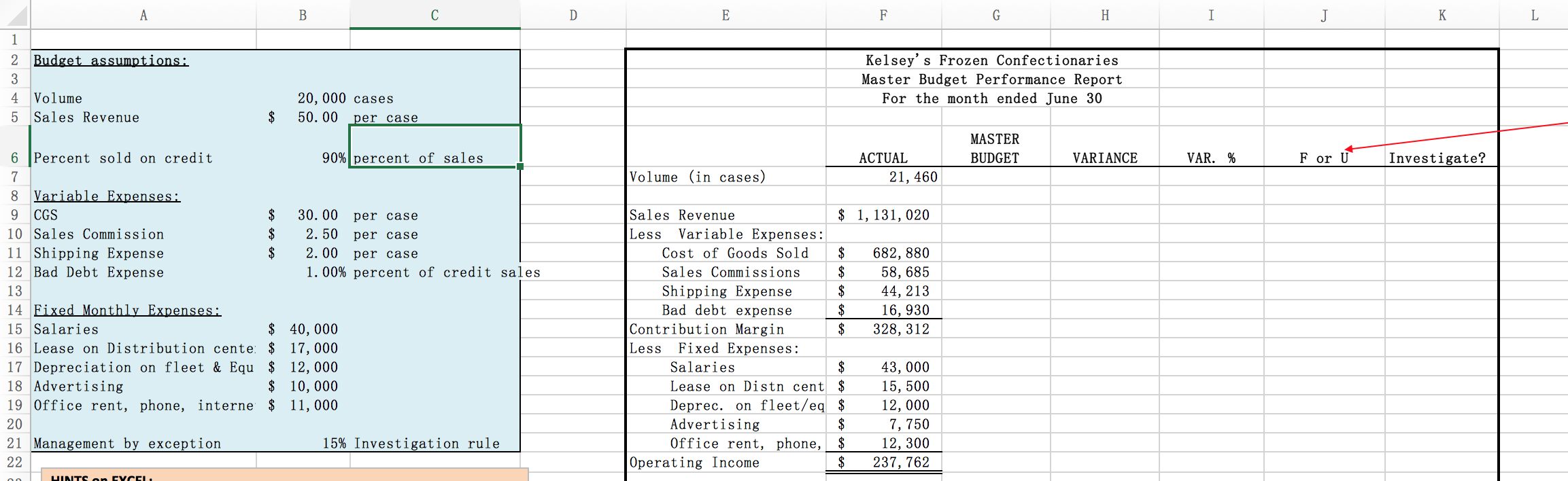
1) Use the budget assumptions, along with Excel formulas, to populate the Master Budget column. Note: Your formulas must work such that if ANY of the budget assumptions change, the new assumptions ripple through the entire budget. Part of your grade will be based on whether you correctly formulate the cells. Do NOT TYPE A NUMBER IN ANY CELL!!!

2) Use a formula to calculate the variance in cell H7: (Actual Budget). Copy and paste (or use the fill handle to drag) the formula to the rest of the cells in the column. Leave as positive or negative, rather than absolute values.

3) Use a formula to calculate the Variance percentage. NOTE: The percentage is the variance as a percent of the Master Budget. Copy and paste (or drag) the formula to the rest of the cells in the column

4) Format cells appropriately. Attention to detail makes a report look more professional. (For example, percentages shown as %, dollar signs using the accounting or currency format, underlines and double underlines where appropriate, zero decimal places for dollar amounts, etc.,).

5) Use the If statement function to show the variances as U or F. The If statement can be found under Formulas, Logical. Example: =IF(H7>=0,"F","U"). This formula means: If cell H7>0 or H7=0, then mark as F; If not greater than or equal to 0, mark as U. Be careful with revenues and expense variances since they should be opposite of one another. ALSO- The formula you use should mark any variance of 0 as an F since a zero variance means that budget expectations have been met. After using the function, check each line to make sure it is going in the direction you believe it should go.

6) Check your answers using the following check figures: Budgeted CM= $301,000; Budgeted Op Inc. = $211,000; Variance for Commissions = $8,685; Variance percentage for Commissions = 17.4 %, Unfavorable.

7) Use management by exception to determine which variances to investigate. HINT: In column K, use the If function, along with Absolute value function to find the variances that are larger than the decision rule. Also, since the decision rule is in B21 and you want Excel to always compare to B21, you need to make it an absolute reference: $B$21.

For example, =IF(ABS(I7)>($B$21),"yes","no"). After using the function, check each line to see whether your formula worked properly.

8) Use the Conditional Formatting feature to automatically highlight any variance that says "yes" to investigate. First, select all of the answers in the "investigate?" column with your cursor. Next select "Conditional formatting" from the home tab on the ribbon. From the drop-down choices select "highlight cells rules" then "Text that contains....". A dialogue box will open. Type in "yes" as the text you want. Leave the default highlight color, or choose a different color from the options listed. Then click OK. Notice how every cell containing "yes" is now highlighted!

9) Center the U/F and Yes/No in the middle of the columns for easier readability.

10) Now check to see if everything ripples through the budget if you change an assumption. Try changing the assumed sales volume to 20,500 and Shipping expense to $2.10 per case. You should have a new total variance for operating income of $21,287, 9.8% variance, F, No.

11) Change the sales volume assumption back to $20,000 and the shipping expense assumption back to $2.00 before continuing.

2 Budget assumptions: Kelsey's Frozen Confectionaries Master Budget Performance Report For the month ended June 30 4 Volume 5 Sales Revenue 20,000 cases 50.00 per case $ MASTER BUDGET 6 Percent sold on credit 90% percent of sales VARIANCE VAR. % For U Investigate? ACTUAL 21, 460 Volume (in cases) 1, 131, 020 8 Variable Expenses: 9 CGS $ 30.00 per case 10 Sales Commission $ 2.50 per case 11 Shipping Expense 2.00 per case 12 Bad Debt Expense 1.00% percent of credit sales 13 14 Fixed Monthly Expenses: Salaries $ 40,000 16 Lease on Distribution cente: $ 17,000 17 Depreciation on fleet & Equ $ 12,000 18 Advertising $ 10,000 19 Office rent, phone, interne $ 11,000 682, 880 58,685 44, 213 16, 930 328, 312 Sales Revenue $ Less Variable Expenses: Cost of Goods Sold $ Sales Commissions $ Shipping Expense Bad debt expense $ Contribution Margin Less Fixed Expenses: Salaries Lease on Distn cent $ Deprec. on fleet/eq $ Advertising $ Office rent, phone, $ Operating Income $ 43,000 15,500 12,000 7, 750 12,300 237, 762 20 21 Management by exception 15% Investigation rule 22 VINTS on CYCEL, Kelsey's Frozen Confectionaries Fexible Budget Performance Report For the month ended June 30 FLEXIBLE BUDGET ACTUAL MASTER BUDGET