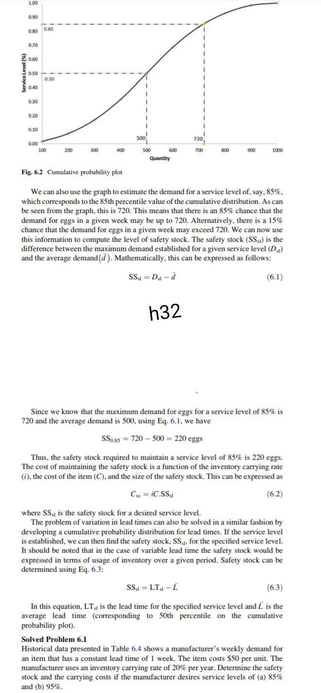
1.00 0.90 0.80 0.85 0.70 0.60 ervice Level (%) 0.50 0.50 0.40 0.30 0.20 0.10 720 0.00 100 200 300 400 700 800 900 1000 500 600 Quantity Fig. 6.2 Cumulative probability plot We can also use the graph to estimate the demand for a service level of, say, 85%, which corresponds to the 85th percentile value of the cumulative distribution. As can be seen from the graph, this is 720. This means that there is an 85% chance that the demand for eggs in a given week may be up to 720. Alternatively, there is a 15% chance that the demand for eggs in a given week may exceed 720. We can now use this information to compute the level of safety stock. The safety stock (SS,1) is the difference between the maximum demand established for a given service level (D1) and the average demand(). Mathematically, this can be expressed as follows: SS=D-d (6.1) h32 Since we know that the maximum demand for eggs for a service level of 85% is 720 and the average demand is 500, using Eq. 6.1, we have SS0.45 = 720 - 500 = 220 eggs Thus, the safety stock required to maintain a service level of 85% is 220 eggs. The cost of maintaining the safety stock is a function of the inventory carrying rate (i), the cost of the item (C), and the size of the safety stock. This can be expressed as Css=iC.SS. (6.2) where SS, is the safety stock for a desired service level. The problem of variation in lead times can also be solved in a similar fashion by developing a cumulative probability distribution for lead times. If the service level is established, we can then find the safety stock, SS, for the specified service level. It should be noted that in the case of variable lead time the safety stock would be expressed in terms of usage of inventory over a given period. Safety stock can be determined using Eq. 6.3: SS=LT-I (6.3) In this equation, LT, is the lead time for the specified service level and I is the average lead time (corresponding to 50th percentile on the cumulative probability plot). Solved Problem 6.1 Historical data presented in Table 6.4 shows a manufacturer's weekly demand for an item that has a constant lead time of 1 week. The item costs $50 per unit. The manufacturer uses an inventory carrying rate of 20% per year. Determine the safety stock and the carrying costs if the manufacturer desires service levels of (a) 85% and (b) 95%