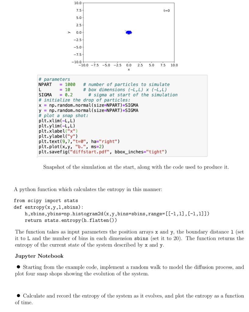
10.0 7.5 t=0 5.0 2.5 0.0 -2.5 -5.0 -7.5 - 10.0 -10.0 -7.5 -5.0 -2.5 0.0 2.5 5.0 7.5 10.0 x # parameters NPART = 1000 # number of particles to simulate L = 10 # box dimensions (LL) X (-L,L) SIGMA = 0.2 # sigma at start of the simulation # initialize the drop of particles: x = np. random.normal(size=NPART) *SIGMA y = np. random.normal(size NPART) SIGMA # plot a snapshot: plt.xlim(-L,L) plt.ylim(-L,L) plt.xlabel("x") plt.ylabel("/") plt.text(9,7,"t=0", ha="right") plt.plot(x,y, ".", ms=2) plt. savefig("diffstart.pdf", bbox_inches="tight") Snapshot of the simulation at the start, along with the code used to produce it. A python function which calculates the entropy in this manner: from scipy import stats def entropy(x,y,l,sbins): h,xbins,ybins=np.histogram2d (x,y,bins=sbins, range=[(-1,1],[-1,1]]) return stats. entropy (h. flatten() The function takes as input parameters the position arrays x and y, the boundary distance 1 (set it to L and the number of bins in each dimension sbins (set it to 20). The function returns the entropy of the current state of the system described by x and y. Jupyter Notebook Starting from the example code, implement a random walk to model the diffusion process, and plot four snap shops showing the evolution of the system. Calculate and record the entropy of the system as it evolves, and plot the entropy as a function of time. 10.0 7.5 t=0 5.0 2.5 0.0 -2.5 -5.0 -7.5 - 10.0 -10.0 -7.5 -5.0 -2.5 0.0 2.5 5.0 7.5 10.0 x # parameters NPART = 1000 # number of particles to simulate L = 10 # box dimensions (LL) X (-L,L) SIGMA = 0.2 # sigma at start of the simulation # initialize the drop of particles: x = np. random.normal(size=NPART) *SIGMA y = np. random.normal(size NPART) SIGMA # plot a snapshot: plt.xlim(-L,L) plt.ylim(-L,L) plt.xlabel("x") plt.ylabel("/") plt.text(9,7,"t=0", ha="right") plt.plot(x,y, ".", ms=2) plt. savefig("diffstart.pdf", bbox_inches="tight") Snapshot of the simulation at the start, along with the code used to produce it. A python function which calculates the entropy in this manner: from scipy import stats def entropy(x,y,l,sbins): h,xbins,ybins=np.histogram2d (x,y,bins=sbins, range=[(-1,1],[-1,1]]) return stats. entropy (h. flatten() The function takes as input parameters the position arrays x and y, the boundary distance 1 (set it to L and the number of bins in each dimension sbins (set it to 20). The function returns the entropy of the current state of the system described by x and y. Jupyter Notebook Starting from the example code, implement a random walk to model the diffusion process, and plot four snap shops showing the evolution of the system. Calculate and record the entropy of the system as it evolves, and plot the entropy as a function of time