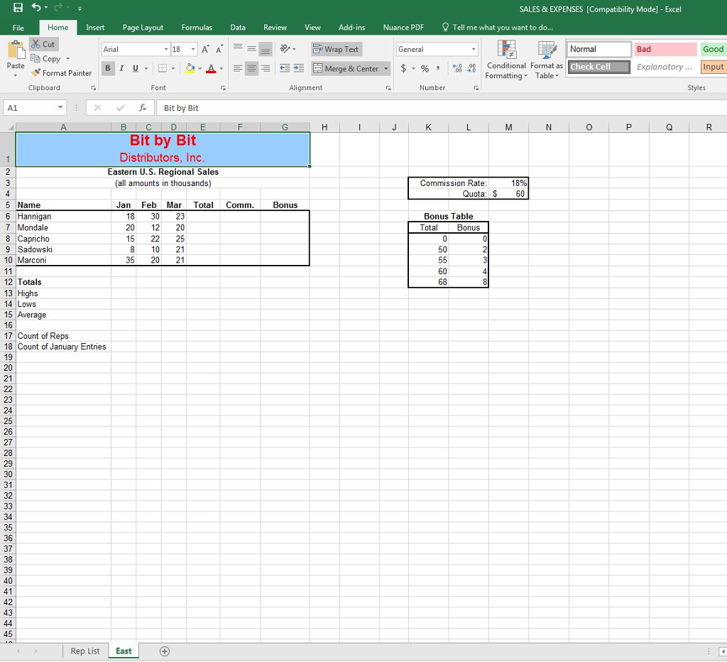
17. In the East sheet, do the following:

In the range E6:E10, calculate the total of the January March sales.

Calculate commissions in column F (F6:F10), as follows: If the sales total (in column E) exceeds the quota in cell N4, the total should be multiplied by 18%. If not, Below Q should appear in the cell.

In the formula, refer to the commission rate of 18% and the quota of 60 by name, not by cell address or value.

Once the formula has been entered into cell F6, Autofill it through cell F10.

In the range G6:G10, calculate the bonus of each rep, based on the contents of the Bonus table in K8:L12. If the Total amount in column E is less than 50, the bonus is 0. If the Total amount is greater than or equal to 50 and less than 55, the Bonus amount is 2, and so forth.

Do not use an If statement or nested If statements to calculate the bonuses, and do not perform the calculations manually.

In the range B13:E15, calculate the high, low, and average sales for each column.

In cell B17, calculate the number of reps (listed in column A).

In cell B18, calculate the number of January values in column B.

Add the following comment to cell E6:

The high sales are due to Hannigans new high protein diet.

Display the comment indicator in cell E6, with the comment appearing only when the cell pointer is positioned on the cell.

Replace all borders in the East sheet that may have been lost due to Autofilling.

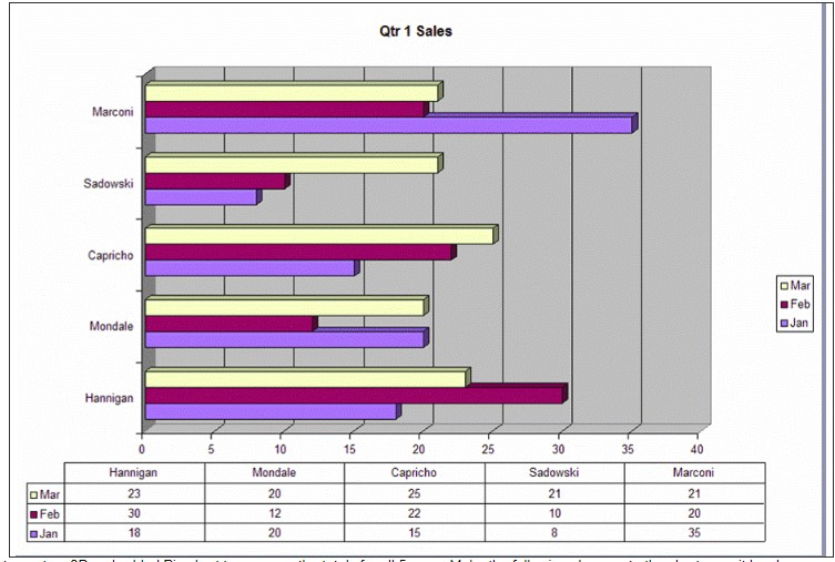
18. Create a three-dimensional Bar chart to compare the January March sales amounts for the 5 sales reps in the East sheet.

Create the chart on a separate sheet named Q1 Sales Chart.

Below the chart, add a data table that details the exact values.

Add Qtr 1 Sales as the chart title.

Change the high Y-axis value to 40.

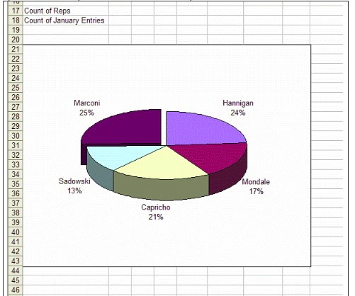
19. In the East sheet, create a 3D embedded Pie chart to compare the totals for all 5 reps. Make the following changes to the chart once it has been created:

Display the rep name and percent next to each pie piece.

Remove the legend and default chart title.

Place the chart below the data, beginning in row 21.

Elevate the 3-D view of the pie to 25.

Explode the Marconi piece of the pie, so that its separated from the rest of the pie.

SALES & EXPENSES [Compatibility Mode] - Excel File Home Insert Page Layout Formulas Data Review View Add-ins Nuance PDF Tell me what you want to do... Wrap Text Normal | Paste 3 ? o-a-- ?Merge & Center ? $ ? 96 , .00 o: Conditional Format as C Formatting Table u- Check Cell Explanatory... Input Format Painter Clipboard Font Alignment Number Styles >K Bit by Bit B C D E Bit by Bit Distributors, Inc Eastern U.S. Regional Sales (all amounts in thousands) 18% Quota: S 60 Commission Rate 5 Name 6 Hannigan 7 Mondale 8 Capricho 9 Sadowski 10 Marconi Jan Feb Mar Total Comm Bonus 18 30 23 20 12 20 15 22 25 8 1021 35 20 21 Bonus Table Tota Bonus 50 12 Totals 13 Highs 14 Lows 15 Average 16 17 Count of Reps 18 Count of January Entries 19 20 21 68 23 24 25 26 27 28 29 30 31 32 35 36 37 38 39 40 41 42 43 45 Rep List East