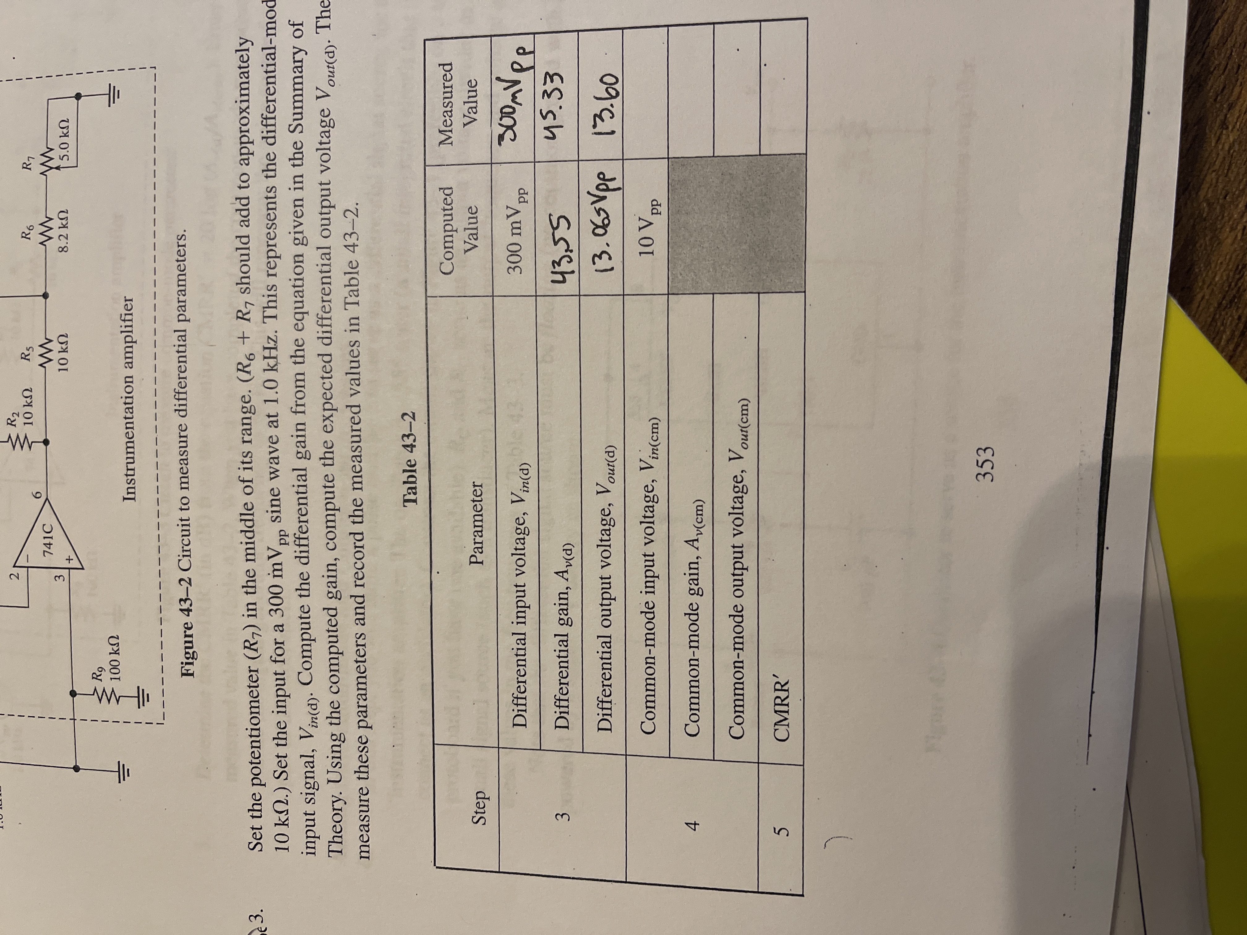
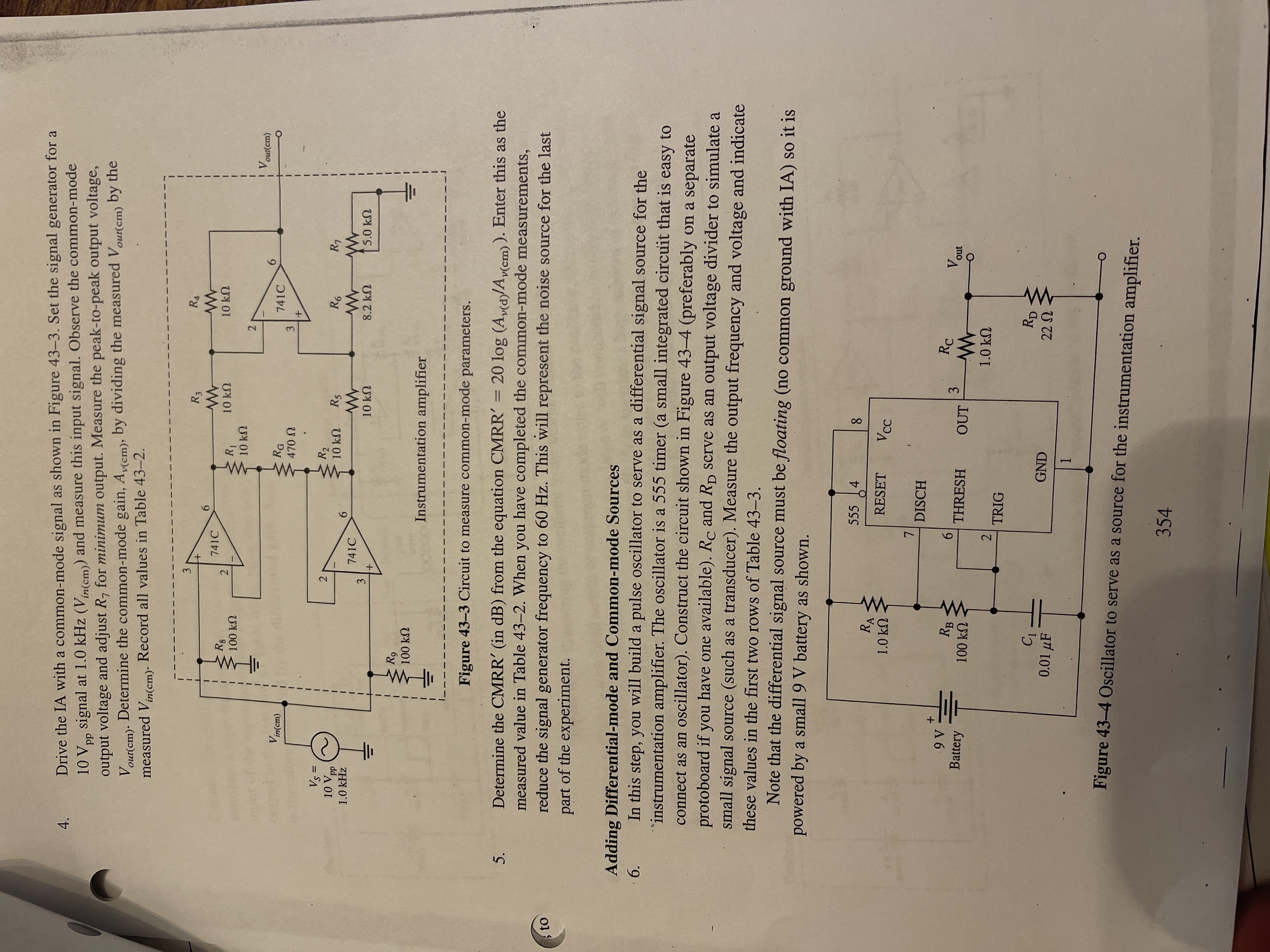
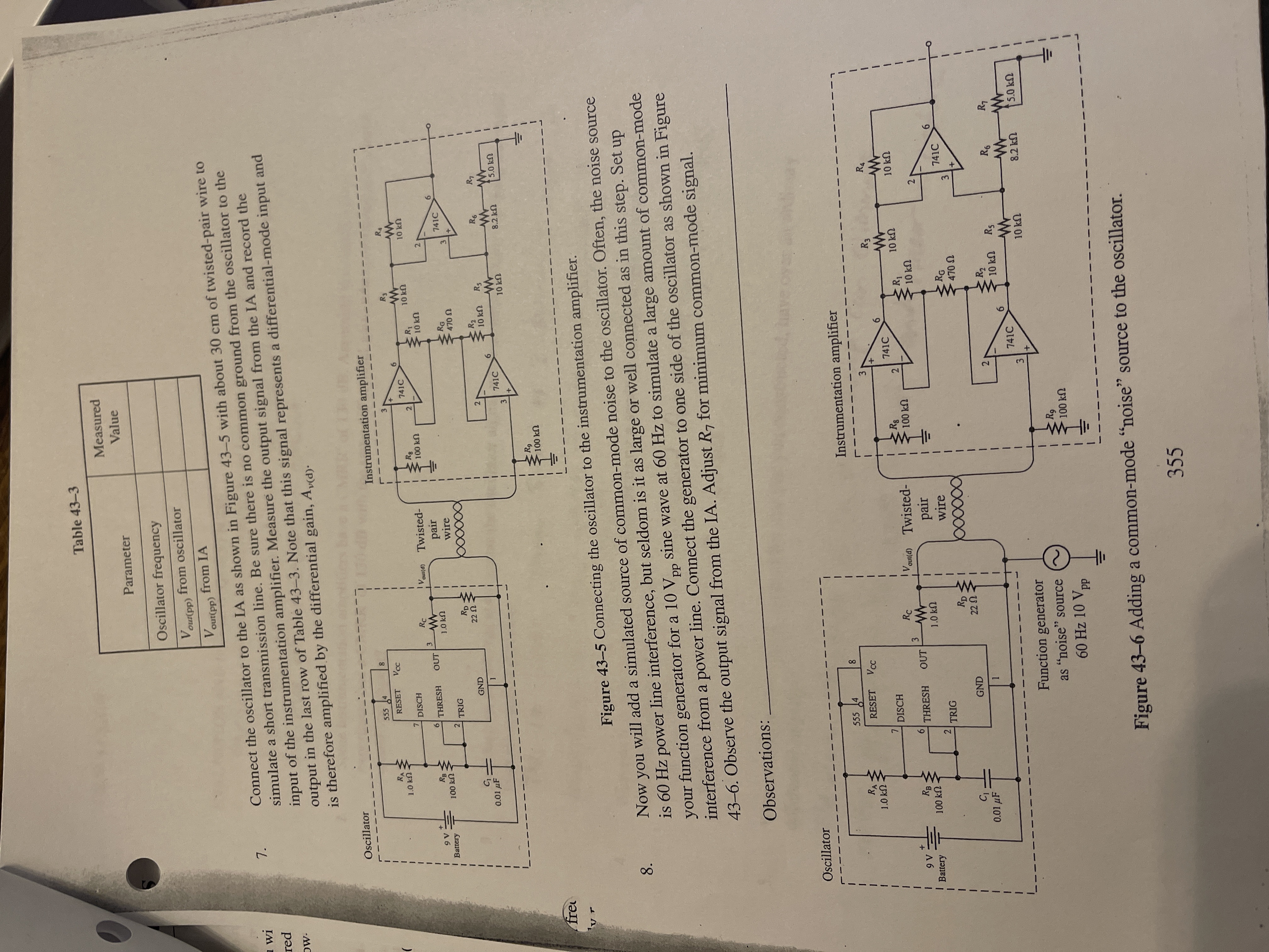
2 2R2 10 kn R5 R6 R7 6 741C W 10 kn 8.2 kn 5.0 kn -100 kn Instrumentation amplifier Figure 43-2 Circuit to measure differential parameters. E 3. Set the potentiometer (R7) in the middle of its range. (R6 + R7 should add to approximately 10 kn.) Set the input for a 300 m Vpp sine wave at 1.0 KHz. This represents the differential-mo input signal, Vin(@). Compute the differential gain from the equation given in the Summary of Theory. Using the computed gain, compute the expected differential output voltage Vour(a). The measure these parameters and record the measured values in Table 43-2. Table 43-2 Computed Measured Step Parameter Value Value Differential input voltage, Vinca) 300 mvpp 300 mupp Differential gain, Av(d) 43,55 45.33 w Differential output voltage, Vour(d) 13. 065 Upp 13.60 Common-mode input voltage, Vin(cm) 10 Vpp 4 Common-mode gain, Av(cm) Common-mode output voltage, Vour(cm) CMRR' 353Drive the IA with a common-mode signal as shown in Figure 43-3. Set the signal generator for a 4. 10 Vpp signal at 1.0 KHz (Vin(cm)) and measure this input signal. Observe the common-mode output voltage and adjust R, for minimum output. Measure the peak-to-peak output voltage, Your(cm). Determine the common-mode gain, Av(cm), by dividing the measured Vour(cm) by the measured Vin(cm)- Record all values in Table 43-2. R3 RA 6 741C W Rg 10 kn 10 kn 100 kn 10 KO Vour(cm) 6 Vin(cm) RG 741C - 470 VS = 2 2R2 10 VD 10 kn R5 R6 1.0 KHz 16 741C 10 kn 8.2 kn 5.0 kn Kg 100 kn Instrumentation amplifier Figure 43-3 Circuit to measure common-mode parameters. 5. Determine the CMRR' (in dB) from the equation CMRR' = 20 log (Ay(d)/Av(cm) ). Enter this as the measured value in Table 43-2. When you have completed the common-mode measurements, to reduce the signal generator frequency to 60 Hz. This will represent the noise source for the last part of the experiment. Adding Differential-mode and Common-mode Sources 6. In this step, you will build a pulse oscillator to serve as a differential signal source for the instrumentation amplifier. The oscillator is a 555 timer (a small integrated circuit that is easy to connect as an oscillator). Construct the circuit shown in Figure 43-4 (preferably on a separate protoboard if you have one available). Rc and RD serve as an output voltage divider to simulate a small signal source (such as a transducer). Measure the output frequency and voltage and indicate these values in the first two rows of Table 43-3. Note that the differential signal source must be floating (no common ground with IA) so it is powered by a small 9 V battery as shown. 555 RA 1.0 kQ RESET Vcc DISCH 9V RBS RC Battery V out 100 kn THRESH 3 OUT -O 2 1.0 kQ TRIG CI RDS 0.01 UF GND 220 5 Figure 43-4 Oscillator to serve as a source for the instrumentation amplifier. 354Table 43-3 Measured Parameter Value Oscillator frequency Vour(pp) from oscillator Vour(pp) from LA 7. Connect the oscillator to the IA as shown in Figure 43-5 with about 30 cm of twisted-pair wire to wi simulate a short transmission line. Be sure there is no common ground from the oscillator to the red input of the instrumentation amplifier. Measure the output signal from the IA and record the output in the last row of Table 43-3. Note that this signal represents a differential-mode input and is therefore amplified by the differential gain, Avcd). Oscillator $55 4 Instrumentation amplifier RESET VCC RA DISCH 41C KC Twisted- R8 100 k ER Oks THRESH OUT 00 kn LOKS pair 10 KO TRIG wire 741C Xxx 470 GND 202 0.01 HF T 2 10 Rs K6 741C 10 kS 8.2 kn 15.0kn free 100 kn Figure 43-5 Connecting the oscillator to the instrumentation amplifier. 8. Now you will add a simulated source of common-mode noise to the oscillator. Often, the noise source is 60 Hz power line interference, but seldom is it as large or well connected as in this step. Set up your function generator for a 10 Vpp sine wave at 60 Hz to simulate a large amount of common-mode interference from a power line. Connect the generator to one side of the oscillator as shown in Figure 43-6. Observe the output signal from the IA. Adjust R7 for minimum common-mode signal. Observations: Oscillator 5554 Instrumentation amplifier 1.0 kn S RESET VCC DISCH R3 RA 741C AM RC 9V Voul(d) Twisted- R1 10 kn Battery THRESH OUT 100 k 10 kQ 100 kn 1.0 kn pair 10 KO TRIC wire 6 AG 741C GND 22 0 470 0 0.01 LLF 5 1 10 kn RS R6 R1 741C AM Function generator 10 kn 3.2 kn 5.0 kn as "noise" source Rg 60 Hz 10 Vpp 100 k Figure 43-6 Adding a common-mode "noise" source to the oscillator. 355