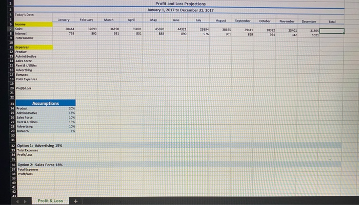
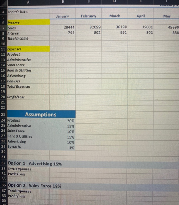
2. Fill the Total Income, Total Expenses, and Profit/Loss rows with Yellow (through column N).

3. Under Income, indent the two income categories two spaces (Sales and Interest). Under Expenses, indent the six expense categories two spaces.

4. Under Assumptions, insert a blank row above Bonus % and type in Target for Bonus, then next to it in B29 type in $35,000.

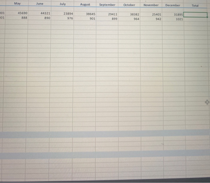
5. Using a function, calculate the Total Sales and Total Interest for the year.

6. Using a formula, calculate the Total Income for January (Sales plus Interest), and copy this across for the remaining months and year total.

7. Calculate the projected expenses (rows 12 through 16 excluding Bonuses) which are based upon the percentages under the assumptions as a portion of the Sales amount which appears under Income. Starting with the Product expenses for January, you will multiply the Sales for January by the Product % under assumptions. You will then copy this formula across for the additional months. Lesson 3, P a g e | 2 (In the original formula, you will need to use absolute and relative referencing. Note: If any of these values are $0, then you didnt use the absolute referencing correctly.)

8. Continue calculating the projected expenses for the remaining expense categories, excluding Bonuses (Administrative through Advertising). As above, you will calculate the amount for January, then copy across to the other months.

9. To calculate the Bonuses for January (row 17), you will use the IF function to compare the January Sales (B7) to the Target for Bonus amount (B29) under Assumptions. If the January Sales meets or exceeds the Target, then they will get a % of the sales as indicated under Assumptions (multiply the % for Bonuses (B30) by the Sales (B7)). If they dont meet the sales amount, then they get $0. Use Absolute and Relative Referencing. Note: It is possible for some of these results to be $0.

10. Copy the Bonuses formula across for the remaining months.

11. Use a function to calculate the total for each of the expense categories (column N) (sum up each row).

12. Use a function to calculate the Total Expenses for January, and copy this across for the additional months and the total for the year.

13. Calculate Profit/Loss row for the months and year by subtracting Total Expenses from Total Income.

14. Format numbers using Accounting Style for the top rows of each of the Income, Expenses, and the Total rows for each in addition to Profit/Loss rows (7, 9, 12, 18, & 20). Format remaining Income and Expense values to Comma Style.

15. Perform What-If Analysis by changing the Advertising % under Assumptions from 10% to 15%. Copy the new Total Expenses and Profit/Loss rows and paste them under the Option1 Heading (rows 34 and 35). Note: You need to Paste Special and use Values and Number formats.

16. Change the Advertising % under assumptions back to 10%. (Be sure the values under Option 1 do not change).

17. Perform What-If Analysis again, this time by changing the Sales Force % under Assumptions (B26) from 10% to 18%. Copy the Total Expenses and Profit/Loss rows and paste them under the Option 2 Heading (rows 38 & 39). See note in step 15

18. Change the Sales Force back to 10%

19. Use a function in cell B4 to display the current date. (you may need to format so that only the date appears)

2 Profit and Loss Projections January 1, 2017 to December 31, 2017 February March April May June August September October November December Total 32099 892 36118 991 35001 801 45690 888 44121 190 23894 976 38545 901 29411 899 2182 964 25401 942 Today's Date: Manuary Income 7 Sales 28444 Interest 795 9 Total income FD 11 Expenses 12 Product 13 Administrative 14 Salesforce 15 Rent Us 16 Adverthing 17 Banuses 18 Total Experts 19 20 Preless 21 22 21 Assumptions 24 Product 2015 25 Admite 15 26 Salesforce 10% 27 Rent & Us 15% 28 Advertising 10N 29 Bonus IN 30 31 32 Option 1: Advertising 15% 33 Total Expenses 34 Profit/Less 35 36 Option 2: Sales Force 18% 37 Total Expenses 1 Prof/loss 41 Profit & Loss + 2 Profit and Loss Projections Jan 1, 2017 10 December 31, 2017 4 Today's Date ary February March May June October November Tos 28 795 31099 92 361 991 35001 101 45690 4632 90 23894 976 25401 942 901 164 1021 Inc Soes interest 9 Toluce 20 11 Eps 12 Product 13 Admiroove 14 Serfare 15 New 16 Advertising 17 Bonus 13 20 Proton 21 Assumptions 20 Predat 25 Admirative 20N 15% 10% 15 10N IN 27 Rent 20 Avrig 20 Bonus 20 Option 1: Advertising 15% 3 Total 34 Pro Option 2: Salesforce 18% 37 Total penses Profile . B February March April May 32099 892 36198 991 35001 801 45690 888 4 Today's Date: 5 January 6 Income 7 Sales 28444 8 Interest 795 9 Total Income 10 11 Expenses 12 Product 13 Administrative 14 Sales Force 15 Rent & Utilities 16 Advertising 17 Bonuses 18 Total Expenses 19 20 Profit/Loss 21 22 23 Assumptions 24 Product 20% 25 Administrative 15% 26 Sales Force 10% 27 Rent & Utilities 15% 28 Advertising 10% 29 Bonus % 1% 30 31 32 Option 1: Advertising 15% 33 Total Expenses 34 Profit/Loss 35 36 Option 2: Sales Force 18% 37 Total Expenses 33 Profit/Loss 39 May June July August September October November December Total 001 301 45690 888 44321 890 23894 976 38645 901 29411 899 38382 964 25401 942 31895 1021 +