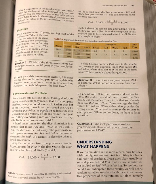
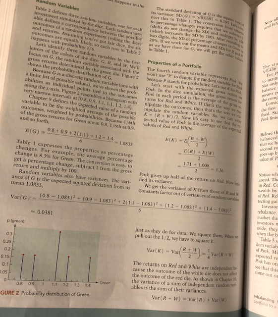
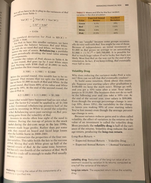
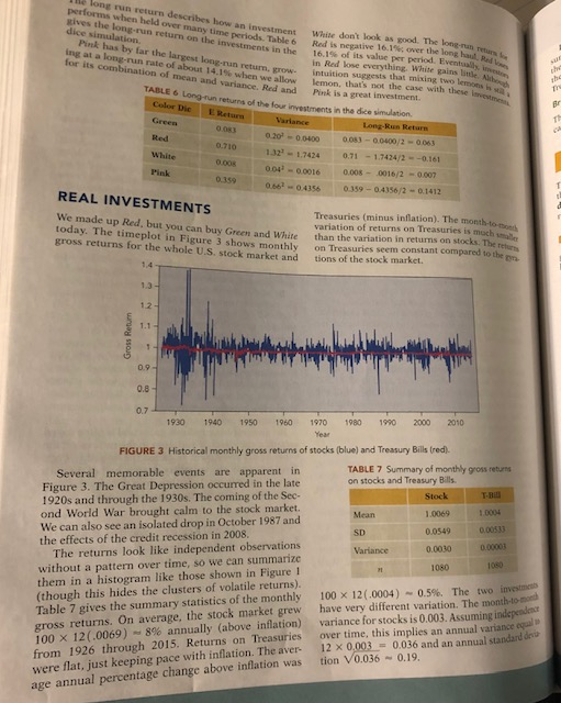
2) Is Pink the best mix of Red and White? There's no rule that says a portfolio has to be an equal mix of two investments.

(a) Find the mean and variance of a portfolio that has 60% invested in White and 40% invested in Red.

(b) Does the portfolio in (a) outperform Pink in the long run?

(c) How might you find a better mixture of Red and White?

3) The example portfolio pink mixes Red and White. Might an investment that mixed Green and Red perform better?

a) Find the mean and variance of a portfolio that mixes half Red and half Green.

b) Does this new mixture outperform Pink in the long run?

4) A portfolio can contain more than two items, such as a mixture of Red, White and Green. Consider the portfolio that has 40% Red, 50% Green, and 10% White.

a) Find the mean and variance of this portfolio

b) Compare the long-run performance of this portfolio to a Pink.

C) Is this the best mixture of the three investments, from a long-run point of view? (keep all of the shares between 0 and 1.)

5) Red is artificial; we dont know an investment that would work so well if paired with returns on Treasures (White). What other attribute of the simulation is artificial? (Hint: This attribute makes it easy to find the variance of Pink)

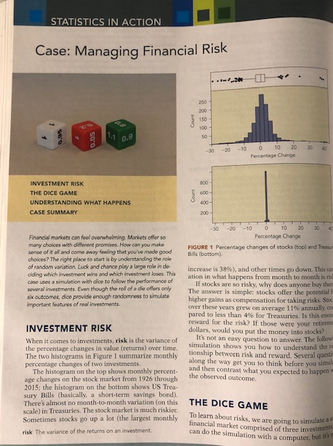
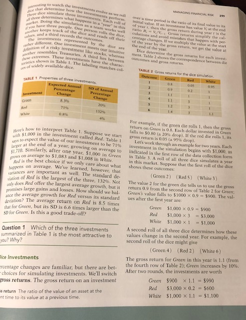
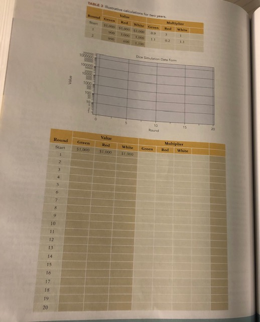
STATISTICS IN ACTION Case: Managing Financial Risk 150 30 20-10 0 10 20 30 Percentage Change 800 INVESTMENT RISK THE DICE GAME UNDERSTANDING WHAT HAPPENS CASE SUMMARY 200 30 -20 10 10 20 30 Percentage Change Financial markets can feel overwhelming. Markets offer so many choices with different promises.How can you make sense of it all and come away feeling that you've made good choices? The right place to start is by understanding the role ofrandom variation. Luck and chance lay aagerindo ciding which investment wins and which investment loser. This case uses a simulation with dice to follow the performance of several investments. Even though the roll of a die offers only six outcomes, dice provide enough randomness to simulate FIGURE 1 Percentage changes of stocks (top) and Treasu Bills (bottom) increase is 38%), and other times go down. This vz ation in what happens from month to month is ris If stocks are so risky, why does anyone buy then The answer is simple: stocks offer the potential f as compensation for taking risks. Sto higher gains over these years grew on average 11% annually, co pared to less than 4% for Treasuries. Is this enou reward for the risk? If those were your dollars, would you put the money into stocks? INVESTMENT RISK It's not an easy question to answer. The followi When it comes to investments, risk is the variance of the percentage changes in value (returns) over time Simulation shows you how to understand the re The two histograms in Figure 1 summarize monthly tionship between risk and reward. Several questi percentage changes of two investments. along the way get you to think before you siml and then contrast what The histogram on the top shows monthly percent- age changes on the stock market from 1926 through 2015; the histogram on the bottom shows US Trea- sury Bills (basically, a short-term savings bond). There's almost no month-to-month variation (on this scale) in Treasuries. The stock market riskier. Sometimes stocks go up a lot (the largest monthly risk The variance of the returns on an investment you expected to happen v the observed outcome THE DIC To learn about ri t is much riskier. To learn about risks, we are going to simulate ats financial can do the simulation with a computer market comprised of three investment but it's n Scar $1,000 $1,000 $1.000 09 Green Red White Gren Multiper T011 02 11 Dice Smulation Dats Fom 10 15 Value RoundG White Red White Start S1,000 $1,000 S1,000 10 12 13 14 17 18 19 20 MANAGING FINANCIAL RISK track of the results after two "years. In the second year, Red has gross return s return 0.2 and bhxe has the largest value, followed by Green, and White has gross return 1.1. The compounded value the larger version of this table (shown larger th nd hen Red. Use hold the results of your simulation White has gross return 1.1. The compounded value Table 3) to Pink becomes values of the investments on the accom and plot the parvine erid Pink: $2,0000.2.1.1 $1,300 Table 4 shows the sample data after adding Pink in the first two years. (Portfolios that compound in this ona simulation for 20 years, keeping track of the way are said to be rebalanced, a topic we'll discuss in Table 3. Be su vlues in the chart TABLE 4 Expanded data form that includes calculations for P in a couple of pages.) che simulation progresses Roll all three diee to find the me for each year. The Multi Red White Green Red White Pink Pink ross returns in Table 2 deter the value of each invest- Start $1,000 $1,00 $1,000 09 900 3,000 1,000 1.1 02 .1 as the dice are rolled. ion 2 Which of the three investments has t value after 20 years in your simulated Before figuring out how Pink does in the simula- tion, consider this question. Since Pink mixes Red and White, where should it be at the end of the simu lation? Think carefully about this question market? vou pick this investment initially? Having uasched the simulation happen, try to explain why Question 3 How does your group expect Pink his investment won. Was it chance, or something to perform? Will it be better or worse than the at you expect to hold up over the long term? others? A Two-Investment Portfolio Few investors buy just one stock. Putting all of your poney into one company means that if this stumbles, then you Go ahead and fill in the returns and values for Pink. Remember, you don't need to roll the dice again. Use the same gross returns that you already piny have for Red and White. Don't average the final a could lose it all. Rather than bet values for Red and White either: that provides the one company, most investors spread the risk b purchasing portfolios. A portfolio reduces the risk by investing in a variety of stocks rather than just wrong answer. You need to average the returns in each period. When you're done, we have a final question Putting everything into one stock seems very ky. But how can we measure risk? A fourth investment for the dice simulation is a Question 4 Did Pink perform as well portfolio that mixes Red and White, so we'll call it you expected? How would you explain the Pot. The dice can be put away. The previously re- performance of Pink? orded gross returns for Red and White determine the returns for Pink. It's easiest to describe what to do with an example. UNDERSTANDING ing the outcomes from the previous example, he gross return for Pink in the first year is the aver- ge of those for Red and White (3 and 1): If your simulation is like most others, Pink finishes with the highest amount. Red is exciting but has a bad habit of crashing. Green does okay, usually in second place behind Pink, but it's not as interest ing as Pink or Red. White is boring. To see how could have anticipated these results, we will define Pink: $1,000 $2,000 nvestment formed by spreading the invested random variables associat ohey among several stocks, bonds, or accounts Two properties of these random variables, namely, happens in the standard deviation Random Variables Table 2 defines three random varia its variance, SD(G) -V0038T nect this to Table 1. The convers to percentage changes requires th (shifts do not change the SD) and (which increases the SD by 100). After s tment simu by the dice. Each random vari two digits, the efines a correspondence between the a random experiment (rolling each SD of percentage chang the dice) as we have done for G, we will get the 20%. If we work out the means and possible dice and returns. Assuming you've got fair dice, the six in Table outcomes are equally likely, so each row in Table 2 happens with probability Lets identify three random variables by the first letters of the colors of the dice: G, R, and W. Well The fourth r to denote the random focus on G, the random variable associated with the won't use gross returns determined by the green die. shows the probability distribution of G Properties of a Portfolio v0436 h random variable represents Pink P to Figure 2 because P stands for probability. Lets Let's start with the expected Because G is a discrete random variable (one with Pink. In the a finite list of possible values), we've shown the prob Pink in each per abilities as individual points tied to the outcomes turn along the x-axis. Figure 2 resembles a histogram with nipulate very narrow intervals at [ each period is the average of the s for Red and White. If that's the the outcomes, then thats t 1.1, 1.2, 1.4). nipulate the random variables. So Chapter 9 defines the expected value of a random K variable to be the weighted Pin we can x +W) /2. Now it's easy to see that the (R weighted by probabiiage of the possible pected value of Pink is the average of the returns for Green are at 0.8, 1/6th at 0.9, the possible Because 1/6th values of Red and White: of the gross and so forth, balanced 0.8+ 0.9+2(1.1) +12+14 1.0833 E(R) E Table 1 expresses the properties as percenta changes. For example, the hange is 8.3% for Green. The conversion is easy to get a percentage change, subtract 1 from the gross return and multiply by 100 1.71 + 1.008 average percentage Random variables also have variances. The vari- ance of G is the expected squared deviation from its mean 1,0833 Pink gives up half of the return on Red.N find its variance wealth by of Red. Rel tecting gai We get the variance of K from those of R and W Constants factor out of variances of random variable rebalance market dun investors m (0.8 1.083)2+ (0.9 1.083)2 +2(1.1 1.083) (1.2 1.083)+(1.4-1 when the b 0.0381 just as they do for data: We square them. When w pull out the 1/2, we have to square it. Table 5 s dom variab of Pink. Mi 0.3 0.25 0.2 Pink has on The returns on Red and White are independen cause the outcome of the white die does the outcome of the red die. As shown in Chapter I the variance of a sum of independent random1a ables is the sum of their variances come oaut on .05 0.8 0.9 1 1.1 12 1.3 1.4 GURE 2 Probability distribution of Green. ar(W) Var(R + w)-Var(R)+V 303 MANAGING FINANCIAL RSK ue have to do is plug in the variances of Red TABLE S Means and SDs for the four random xpected Annual 8. 3% und While from Table t ariables in the dice simulation Var(K) (Var(R) Var(w)) 1322+0.04 Red 32% 0.436 tandard deviation for Pink is SD(K) 0.66 We say "usually because some groups occasion- ally do very well with Red. You might be one of those Because of independence, an initial investment of $1,000 in Red grows on average to an astonishing Pink to have this smaller variance, we have Ptet For tzin the balance between Red and White. only do we need Red and White, we have to re- the mi of assets. Rebalancing a portfolio periodically dividing the total value among $1,000 x (1.71)20 $45,700,000. It is possible for Red to reach huge values if we're lucky, but that's not likely. Most find Red on the way out by the end of the simulation. In fact, if we keep rolling, Red eventually compnen the values of Pink shown in Table 4. I n round, Red goes up by 3 and White sta Starting with $500 (half of $1,000) in each, mest fall to zero sed. finishes the first round valued at 3(500) 1(500) $2,000 Volatility Drag e second round, this wealth has to be re- holanced. That means that we split the $2,000 so e Why does reducing the variance make Pink a win ner? How can we tell that Red eventually crashes? To build some intuition, think about this exam ple. Suppose your starting salary after graduation i we have $1,000 in each of Red and White. In th und. Red loses 80% of its value and intre by 10%. At the end of the second round, the S100000(to keep the m and you get a 10% raise after a year Your ath easy). Things go goes up aue of Pnk is salary jumps to $110,000. The business does not do so well in the following year and you take a 10% cut. At the end of the second year, your salary is $99,000 Even though the average percentage change is zero (up 10%, down 10%), the variability in the chan 0.2(1,000) +1.1 (1,000)$1,300 Notice what would have happened had we not rebal- anced. The factor 0.2 would be applied to all $1,500 in Red. Continual rebalancing protects half of the in White to avoid the volatility eaves you making 99% of your starting salary You've lost money even though the average percent- age change is zero vealth by investing of Rd. Rebalancing saves past earnings on Red, pro- ecting gains from the volatility of Red Because variance reduces gains and is often called volatility, the effect of variation in the returns on the Investors in stocks often lose sight of the need to rebalance. During the run-up of prices in the stock value of an i nvestment is called the volatility dra murkct during the dot-com surge in the late 1990s, More precisely, the volatility drag is half of the vari netors made huge profits. Rather than put some side, they stayed on board and faced large losses nce of the returns. Volatility drag reduces the av age return, producing the long-run return. when the bubble burst in 2000-2001 Table 5 summarizes the properties of the four ran- Long-Run Return om variables. This table holds the key to the successExpected Annual Return Pk Mixing Red with White gives up half of the apected return of Red. At the Volatility Drag (Annual Variance)/2 Return same time, however. Expected Annual Pok has only one-fourth of the variance of Red. Wel that this trade-off is enough to make Pink usually come out on top. volatility drag Reduction of the long-run value of vestment caused by variation in its returns; computed as one-half the variance of the return elng Hoding the value of the components of a long-run return The expected return minus the volatility drag volatility to a specified mix. Ile long run return performs when held over gives the long-run escribes how an investment White dont look as good. The long-run retu ny time periods. Table 6 Red is negative 16.1%; over the long haul, An a urn on the investments in the Pink has by far the largest long-run 16.1% ofits value per period. Eventuall in Red lose everything. White gains little lemon, that's not the case with these Pink is a great investment. for its combination of itin rate or about 14.1% when we allow of mean and variance. Red and run return.w ntuition suggests that mixing two lermons h tbe TABLE Long-run returns of the four investments in the dice simulation. pr Color Dic E Retr Long-Run Retur 0.083 0.202-00400 0083-00400/2-0063 1.32,-1.7424 0.71-1.7424/2-.0.161 004-00016 0.008-0016/2 -0.007 O.662-0.4356 0.339-0.4356/2-0.1412 Red 0.008 Pink REAL INVESTMENTS Treasuries (minus inflation). The month-tote We made up Red, but today. The timeplo gross returns for the t you can buy Green and White t in Figure 3 shows monthly whole U.S. stock market and variation of returns on Treasuries is moc than the variation in returns on stocks. The returs on Treasuries seem constant compared to the tions of the stock market. 14 1.3 0.8 0.7 1930 1940 1950 1960 197O 1980 990 2000 2010 Year FIGURE 3 Historical monthly gross returns of stocks (blue) and Treasury Bills (red). TABLE 7 Summary of monthly gross returns on stocks and Treasury Bills Several memorable events are apparent in Figure 3. The Great Depression occurred in the late 1920s and through the 1930s. The coming of the Seo ond World War brought calm to the stock market We can also see an isolated drop in October 1987 and the effects of the credit recession in 2008 T-BU Stoc 1.0069 0.0549 0.0030 1.0004 Mean SD Variance The returns look like independent observations without a pattern over time, so we can summarize them in a histogram like those shown in Figure1 (though this hides the clusters of volatile returns). Table 7 gives the summary statistics of the monthly 100 x 12(.0004) ~ 0.5%. The two investmen gross returns 100 x 12(.0069)-8% annually (above inflation) variance for stocks is 0.003. Assuming from 1926 through 2015. Returns on Treasuries over time, this implies an annual variance eqal On average, the stock market grew have very different variation. The month-to ond ing pace with inflation. The aver- 12 x 0,0030.036 and an annual standard dei age annual percentage change above inflation was tion V0.0360.19 STATISTICS IN ACTION Case: Managing Financial Risk 150 30 20-10 0 10 20 30 Percentage Change 800 INVESTMENT RISK THE DICE GAME UNDERSTANDING WHAT HAPPENS CASE SUMMARY 200 30 -20 10 10 20 30 Percentage Change Financial markets can feel overwhelming. Markets offer so many choices with different promises.How can you make sense of it all and come away feeling that you've made good choices? The right place to start is by understanding the role ofrandom variation. Luck and chance lay aagerindo ciding which investment wins and which investment loser. This case uses a simulation with dice to follow the performance of several investments. Even though the roll of a die offers only six outcomes, dice provide enough randomness to simulate FIGURE 1 Percentage changes of stocks (top) and Treasu Bills (bottom) increase is 38%), and other times go down. This vz ation in what happens from month to month is ris If stocks are so risky, why does anyone buy then The answer is simple: stocks offer the potential f as compensation for taking risks. Sto higher gains over these years grew on average 11% annually, co pared to less than 4% for Treasuries. Is this enou reward for the risk? If those were your dollars, would you put the money into stocks? INVESTMENT RISK It's not an easy question to answer. The followi When it comes to investments, risk is the variance of the percentage changes in value (returns) over time Simulation shows you how to understand the re The two histograms in Figure 1 summarize monthly tionship between risk and reward. Several questi percentage changes of two investments. along the way get you to think before you siml and then contrast what The histogram on the top shows monthly percent- age changes on the stock market from 1926 through 2015; the histogram on the bottom shows US Trea- sury Bills (basically, a short-term savings bond). There's almost no month-to-month variation (on this scale) in Treasuries. The stock market riskier. Sometimes stocks go up a lot (the largest monthly risk The variance of the returns on an investment you expected to happen v the observed outcome THE DIC To learn about ri t is much riskier. To learn about risks, we are going to simulate ats financial can do the simulation with a computer market comprised of three investment but it's n Scar $1,000 $1,000 $1.000 09 Green Red White Gren Multiper T011 02 11 Dice Smulation Dats Fom 10 15 Value RoundG White Red White Start S1,000 $1,000 S1,000 10 12 13 14 17 18 19 20 MANAGING FINANCIAL RISK track of the results after two "years. In the second year, Red has gross return s return 0.2 and bhxe has the largest value, followed by Green, and White has gross return 1.1. The compounded value the larger version of this table (shown larger th nd hen Red. Use hold the results of your simulation White has gross return 1.1. The compounded value Table 3) to Pink becomes values of the investments on the accom and plot the parvine erid Pink: $2,0000.2.1.1 $1,300 Table 4 shows the sample data after adding Pink in the first two years. (Portfolios that compound in this ona simulation for 20 years, keeping track of the way are said to be rebalanced, a topic we'll discuss in Table 3. Be su vlues in the chart TABLE 4 Expanded data form that includes calculations for P in a couple of pages.) che simulation progresses Roll all three diee to find the me for each year. The Multi Red White Green Red White Pink Pink ross returns in Table 2 deter the value of each invest- Start $1,000 $1,00 $1,000 09 900 3,000 1,000 1.1 02 .1 as the dice are rolled. ion 2 Which of the three investments has t value after 20 years in your simulated Before figuring out how Pink does in the simula- tion, consider this question. Since Pink mixes Red and White, where should it be at the end of the simu lation? Think carefully about this question market? vou pick this investment initially? Having uasched the simulation happen, try to explain why Question 3 How does your group expect Pink his investment won. Was it chance, or something to perform? Will it be better or worse than the at you expect to hold up over the long term? others? A Two-Investment Portfolio Few investors buy just one stock. Putting all of your poney into one company means that if this stumbles, then you Go ahead and fill in the returns and values for Pink. Remember, you don't need to roll the dice again. Use the same gross returns that you already piny have for Red and White. Don't average the final a could lose it all. Rather than bet values for Red and White either: that provides the one company, most investors spread the risk b purchasing portfolios. A portfolio reduces the risk by investing in a variety of stocks rather than just wrong answer. You need to average the returns in each period. When you're done, we have a final question Putting everything into one stock seems very ky. But how can we measure risk? A fourth investment for the dice simulation is a Question 4 Did Pink perform as well portfolio that mixes Red and White, so we'll call it you expected? How would you explain the Pot. The dice can be put away. The previously re- performance of Pink? orded gross returns for Red and White determine the returns for Pink. It's easiest to describe what to do with an example. UNDERSTANDING ing the outcomes from the previous example, he gross return for Pink in the first year is the aver- ge of those for Red and White (3 and 1): If your simulation is like most others, Pink finishes with the highest amount. Red is exciting but has a bad habit of crashing. Green does okay, usually in second place behind Pink, but it's not as interest ing as Pink or Red. White is boring. To see how could have anticipated these results, we will define Pink: $1,000 $2,000 nvestment formed by spreading the invested random variables associat ohey among several stocks, bonds, or accounts Two properties of these random variables, namely, happens in the standard deviation Random Variables Table 2 defines three random varia its variance, SD(G) -V0038T nect this to Table 1. The convers to percentage changes requires th (shifts do not change the SD) and (which increases the SD by 100). After s tment simu by the dice. Each random vari two digits, the efines a correspondence between the a random experiment (rolling each SD of percentage chang the dice) as we have done for G, we will get the 20%. If we work out the means and possible dice and returns. Assuming you've got fair dice, the six in Table outcomes are equally likely, so each row in Table 2 happens with probability Lets identify three random variables by the first letters of the colors of the dice: G, R, and W. Well The fourth r to denote the random focus on G, the random variable associated with the won't use gross returns determined by the green die. shows the probability distribution of G Properties of a Portfolio v0436 h random variable represents Pink P to Figure 2 because P stands for probability. Lets Let's start with the expected Because G is a discrete random variable (one with Pink. In the a finite list of possible values), we've shown the prob Pink in each per abilities as individual points tied to the outcomes turn along the x-axis. Figure 2 resembles a histogram with nipulate very narrow intervals at [ each period is the average of the s for Red and White. If that's the the outcomes, then thats t 1.1, 1.2, 1.4). nipulate the random variables. So Chapter 9 defines the expected value of a random K variable to be the weighted Pin we can x +W) /2. Now it's easy to see that the (R weighted by probabiiage of the possible pected value of Pink is the average of the returns for Green are at 0.8, 1/6th at 0.9, the possible Because 1/6th values of Red and White: of the gross and so forth, balanced 0.8+ 0.9+2(1.1) +12+14 1.0833 E(R) E Table 1 expresses the properties as percenta changes. For example, the hange is 8.3% for Green. The conversion is easy to get a percentage change, subtract 1 from the gross return and multiply by 100 1.71 + 1.008 average percentage Random variables also have variances. The vari- ance of G is the expected squared deviation from its mean 1,0833 Pink gives up half of the return on Red.N find its variance wealth by of Red. Rel tecting gai We get the variance of K from those of R and W Constants factor out of variances of random variable rebalance market dun investors m (0.8 1.083)2+ (0.9 1.083)2 +2(1.1 1.083) (1.2 1.083)+(1.4-1 when the b 0.0381 just as they do for data: We square them. When w pull out the 1/2, we have to square it. Table 5 s dom variab of Pink. Mi 0.3 0.25 0.2 Pink has on The returns on Red and White are independen cause the outcome of the white die does the outcome of the red die. As shown in Chapter I the variance of a sum of independent random1a ables is the sum of their variances come oaut on .05 0.8 0.9 1 1.1 12 1.3 1.4 GURE 2 Probability distribution of Green. ar(W) Var(R + w)-Var(R)+V 303 MANAGING FINANCIAL RSK ue have to do is plug in the variances of Red TABLE S Means and SDs for the four random xpected Annual 8. 3% und While from Table t ariables in the dice simulation Var(K) (Var(R) Var(w)) 1322+0.04 Red 32% 0.436 tandard deviation for Pink is SD(K) 0.66 We say "usually because some groups occasion- ally do very well with Red. You might be one of those Because of independence, an initial investment of $1,000 in Red grows on average to an astonishing Pink to have this smaller variance, we have Ptet For tzin the balance between Red and White. only do we need Red and White, we have to re- the mi of assets. Rebalancing a portfolio periodically dividing the total value among $1,000 x (1.71)20 $45,700,000. It is possible for Red to reach huge values if we're lucky, but that's not likely. Most find Red on the way out by the end of the simulation. In fact, if we keep rolling, Red eventually compnen the values of Pink shown in Table 4. I n round, Red goes up by 3 and White sta Starting with $500 (half of $1,000) in each, mest fall to zero sed. finishes the first round valued at 3(500) 1(500) $2,000 Volatility Drag e second round, this wealth has to be re- holanced. That means that we split the $2,000 so e Why does reducing the variance make Pink a win ner? How can we tell that Red eventually crashes? To build some intuition, think about this exam ple. Suppose your starting salary after graduation i we have $1,000 in each of Red and White. In th und. Red loses 80% of its value and intre by 10%. At the end of the second round, the S100000(to keep the m and you get a 10% raise after a year Your ath easy). Things go goes up aue of Pnk is salary jumps to $110,000. The business does not do so well in the following year and you take a 10% cut. At the end of the second year, your salary is $99,000 Even though the average percentage change is zero (up 10%, down 10%), the variability in the chan 0.2(1,000) +1.1 (1,000)$1,300 Notice what would have happened had we not rebal- anced. The factor 0.2 would be applied to all $1,500 in Red. Continual rebalancing protects half of the in White to avoid the volatility eaves you making 99% of your starting salary You've lost money even though the average percent- age change is zero vealth by investing of Rd. Rebalancing saves past earnings on Red, pro- ecting gains from the volatility of Red Because variance reduces gains and is often called volatility, the effect of variation in the returns on the Investors in stocks often lose sight of the need to rebalance. During the run-up of prices in the stock value of an i nvestment is called the volatility dra murkct during the dot-com surge in the late 1990s, More precisely, the volatility drag is half of the vari netors made huge profits. Rather than put some side, they stayed on board and faced large losses nce of the returns. Volatility drag reduces the av age return, producing the long-run return. when the bubble burst in 2000-2001 Table 5 summarizes the properties of the four ran- Long-Run Return om variables. This table holds the key to the successExpected Annual Return Pk Mixing Red with White gives up half of the apected return of Red. At the Volatility Drag (Annual Variance)/2 Return same time, however. Expected Annual Pok has only one-fourth of the variance of Red. Wel that this trade-off is enough to make Pink usually come out on top. volatility drag Reduction of the long-run value of vestment caused by variation in its returns; computed as one-half the variance of the return elng Hoding the value of the components of a long-run return The expected return minus the volatility drag volatility to a specified mix. Ile long run return performs when held over gives the long-run escribes how an investment White dont look as good. The long-run retu ny time periods. Table 6 Red is negative 16.1%; over the long haul, An a urn on the investments in the Pink has by far the largest long-run 16.1% ofits value per period. Eventuall in Red lose everything. White gains little lemon, that's not the case with these Pink is a great investment. for its combination of itin rate or about 14.1% when we allow of mean and variance. Red and run return.w ntuition suggests that mixing two lermons h tbe TABLE Long-run returns of the four investments in the dice simulation. pr Color Dic E Retr Long-Run Retur 0.083 0.202-00400 0083-00400/2-0063 1.32,-1.7424 0.71-1.7424/2-.0.161 004-00016 0.008-0016/2 -0.007 O.662-0.4356 0.339-0.4356/2-0.1412 Red 0.008 Pink REAL INVESTMENTS Treasuries (minus inflation). The month-tote We made up Red, but today. The timeplo gross returns for the t you can buy Green and White t in Figure 3 shows monthly whole U.S. stock market and variation of returns on Treasuries is moc than the variation in returns on stocks. The returs on Treasuries seem constant compared to the tions of the stock market. 14 1.3 0.8 0.7 1930 1940 1950 1960 197O 1980 990 2000 2010 Year FIGURE 3 Historical monthly gross returns of stocks (blue) and Treasury Bills (red). TABLE 7 Summary of monthly gross returns on stocks and Treasury Bills Several memorable events are apparent in Figure 3. The Great Depression occurred in the late 1920s and through the 1930s. The coming of the Seo ond World War brought calm to the stock market We can also see an isolated drop in October 1987 and the effects of the credit recession in 2008 T-BU Stoc 1.0069 0.0549 0.0030 1.0004 Mean SD Variance The returns look like independent observations without a pattern over time, so we can summarize them in a histogram like those shown in Figure1 (though this hides the clusters of volatile returns). Table 7 gives the summary statistics of the monthly 100 x 12(.0004) ~ 0.5%. The two investmen gross returns 100 x 12(.0069)-8% annually (above inflation) variance for stocks is 0.003. Assuming from 1926 through 2015. Returns on Treasuries over time, this implies an annual variance eqal On average, the stock market grew have very different variation. The month-to ond ing pace with inflation. The aver- 12 x 0,0030.036 and an annual standard dei age annual percentage change above inflation was tion V0.0360.19