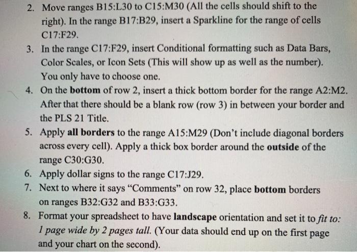
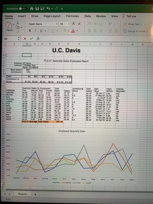
2. Move ranges B15:L30 to C15:M30 (All the cells should shift to the right). In the range B17:B29, insert a Sparkline for the range of cells C17:F29. 3. In the range C17:F29, insert Conditional formatting such as Data Bars, Color Scales, or Icon Sets (This will show up as well as the number). You only have to choose one. 4. On the bottom of row 2, insert a thick bottom border for the range A2:M2. After that there should be a blank row (row 3) in between your border and the PLS 21 Title. 5. Apply all borders to the range A15:M29 (Don't include diagonal borders across every cell). Apply a thick box border around the outside of the range C30:G30. 6. Apply dollar signs to the range C17:J29. 7. Next to where it says "Comments" on row 32, place bottom borders on ranges B32:G32 and B33:G33. 1 Format your spreadsheet to have landscape orientation and set it to fit to: page wide by 2 pages tall. (Your data should end up on the first page and your chart on the second). 8. T 2 3 HHORNOVA AutoSave OFF Home 82 Paste 10 11 Sales 40 1995 12 Bonus 13 14 242522338 15 16 Employee 17 Gabrielle 18 Michell 19 Kyle 20 Courtney 21 Julana 22 Paul 23 Bella 24 Lyuan 25 Caleb 25 Jenny 27 Amy 28 Conor 29 Aedric Commission & 3000 400 40.00 10:00 Base Salary Commission A 20:00 10:00 0.00 Insert Draw Page Layout Edit 16 Shipping UC Devis Address x fx B Open Sans BTU. Sheds Ave Davis, CA 95816 335 10% First 26.93 22.18 42.00 7,14 C D 36.06 38.29 14.87 15.98 # Report E Gebe vanil Fyk Quarterly Sales (in thousands) Total Second Third Fourth Sales 14.23 4.12 8.22 18.34 32.54 7.50 + V V 10 F 11.23 30.50 29.81 11.50 12.87 18.04 15.24 28.41 15.00 20.12 79.67 32.12 22.10 29.41 26.52 21.12 20.65 32.48 53.87 33.33 9.50 119.69 106.50 134.56 56.45 33.12 121,82 45.02 57.34 40.21 23.56 160.13 13.00 33.59 48.20 10.40 40.24 5.99 9.85 22.67 PLS 21 Average Total Sales 12.47 18.50 26.67 38.52 23.51 30 350 $75 $100 $125 $150 $1.00 $5.00 16.50 $8.00 $10.00 $12.50 Gurtny Ala - 53.50 80.56 113.57 49.55 Formulas Y M U.C. Davis G A A Pad A PLS 21 Associate Sales Employees Report V Salary Bonus 47.19 5 53.74 6.5 38.52 8 47.54 1 42.22 6.5 52.168 37.29 8 53.11 10 37.46 5 48 22 8 53 25 12.5 105.19 60.11 8 78.75 29.90 6.5 $97.39 H Commision Data Review View Employee Quartely Sales Uy EE Total Date Salary Hired 52.19 60.24 46.52 48.54 48.72 60.16 45.29 63.11 42.46 56.22 65.75 68.11 36.49 -SondThat Fauth Cale Years WiFvm 28-Jan-17 3.82 27-May-07 23.50 2-Jul-05 15.40 6-May-01 19.55 14-Aug-19 1.27 18-Aug-02 18.27 23-May-09 11.51 24-Dec-12 7.91 29-Jun-07 13.41 29-Oct-12 8.07 19-Mar-11 9.68 7-Nov-88 32.06 20-Apr-94 26.61 Any Training Required? yes yes No yes ves No No No yos No No No yes 2 Wrap Text A Tell me Comer Merge & Center M Adric N