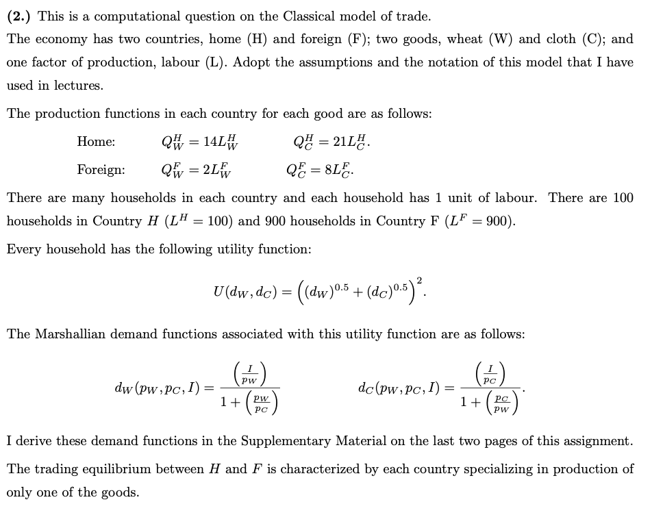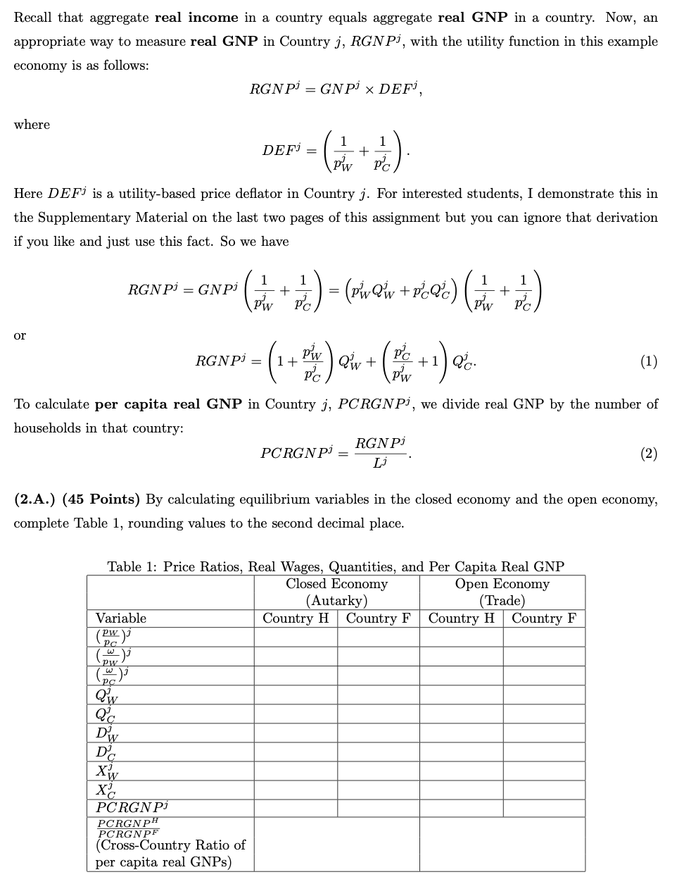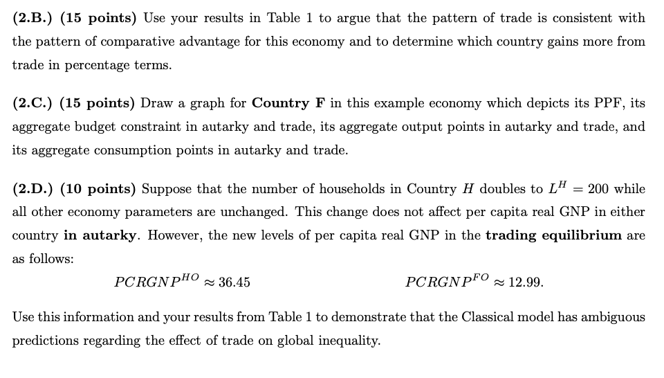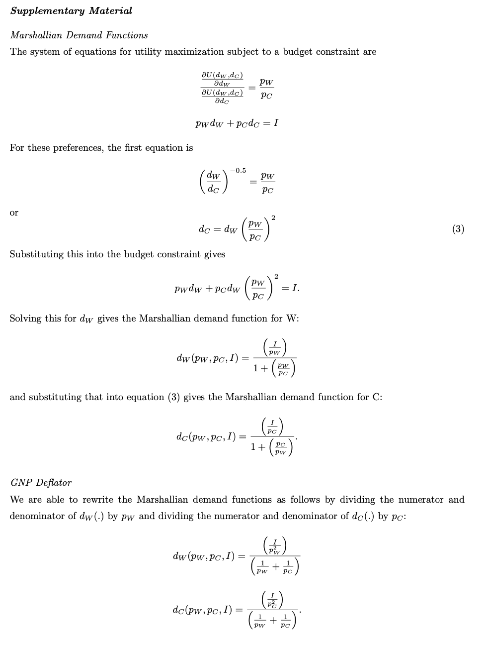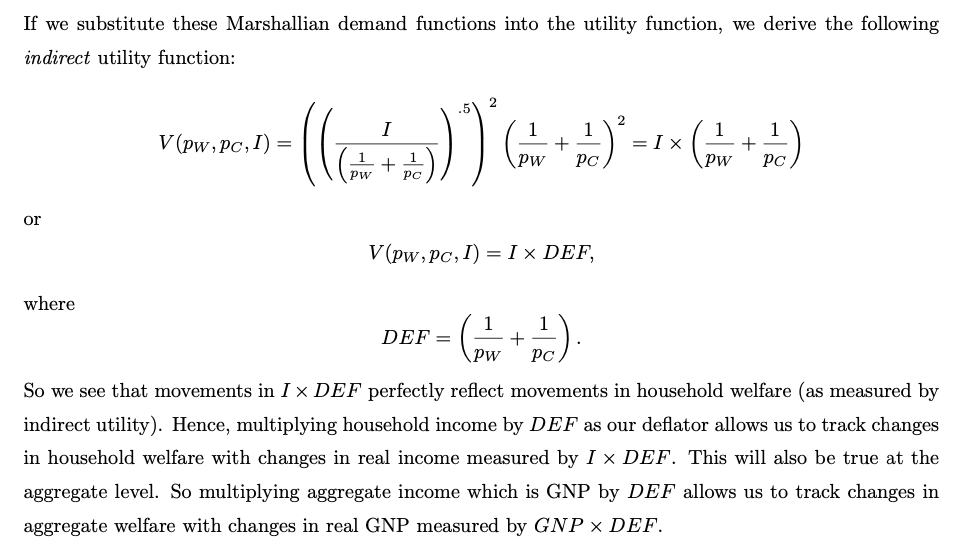
(2.) This is a computational question on the Classical model of trade. The economy has two countries, home (H) and foreign (F); two goods, wheat (W) and cloth (C); and one factor of production, labour (L). Adopt the assumptions and the notation of this model that I have used in lectures. The production functions in each country for each good are as follows: Home: Q# = 14LW Q = 211. Foreign: Q = 2L QE = 8LE There are many households in each country and each household has 1 unit of labour. There are 100 households in Country H (LH = 100) and 900 households in Country F (LF = 900). Every household has the following utility function: U(dw ,dc) = ((dw)0.5 + (dc)0:5)? The Marshallian demand functions associated with this utility function are as follows: (2) PC dw (Pw,pc, 1) = 1+ dc(pw, pc, I) PW PC 1 +( PC Pw I derive these demand functions in the Supplementary Material on the last two pages of this assignment. The trading equilibrium between H and F is characterized by each country specializing in production of only one of the goods. Recall that aggregate real income in a country equals aggregate real GNP in a country. Now, an appropriate way to measure real GNP in Country j, RGNP), with the utility function in this example economy is as follows: RGNP) = GNP > DEF where 1 DEF = + PW Pc) Here DEFi is a utility-based price deflator in Country j. For interested students, I demonstrate this in the Supplementary Material on the last two pages of this assignment but you can ignore that derivation if you like and just use this fact. So we have RGNPi = GNPi Pi ( + ) = (vdw@im +PQ) (2 + 1 PC or RGNPi = PW 1+ + +1 (1) PC) \PW To calculate per capita real GNP in Country j, PCRGNP), we divide real GNP by the number of households in that country: RGN Pi PCRGNP Li (2) (2.A.) (45 Points) By calculating equilibrium variables in the closed economy and the open economy, complete Table 1, rounding values to the second decimal place. Table 1: Price Ratios, Real Wages, Quantities, and Per Capita Real GNP Closed Economy Open Economy (Autarky) (Trade) Variable Country H Country F Country H Country F (Pw PC (wa) Qw QC D' D' Xw X2 PCRGN Pi PCRGNPH PCRGNPF (Cross-Country Ratio of per capita real GNPs) (2.B.) (15 points) Use your results in Table 1 to argue that the pattern of trade is consistent with the pattern of comparative advantage for this economy and to determine which country gains more from trade in percentage terms. (2.C.) (15 points) Draw a graph for Country F in this example economy which depicts its PPF, its aggregate budget constraint in autarky and trade, its aggregate output points in autarky and trade, and its aggregate consumption points in autarky and trade. (2.D.) (10 points) Suppose that the number of households in Country H doubles to LH = 200 while all other economy parameters are unchanged. This change does not affect per capita real GNP in either country in autarky. However, the new levels of per capita real GNP in the trading equilibrium are as follows: PCRGNPHO ~ 36.45 PCRGNPFO 12.99. Use this information and your results from Table 1 to demonstrate that the Classical model has ambiguous predictions regarding the effect of trade on global inequality. Supplementary Material Marshallian Demand Functions The system of equations for utility maximization subject to a budget constraint are au (dw.dc) adw au (dw.de) Pw PC ado pwdw + pcdc = I For these preferences, the first equation is -0.5 dw Pw PC do or 2 ( (3) Pw dc = dw PC Substituting this into the budget constraint gives 2 pw pwdw + pcdw Pc =I. Solving this for dw gives the Marshallian demand function for W: PW dw (Pw, PC, I) 1+ w PC and substituting that into equation (3) gives the Marshallian demand function for C: () dc(pw, pc, I) 1+ PC w GNP Deflator We are able to rewrite the Marshallian demand functions as follows by dividing the numerator and denominator of dw (.) by pw and dividing the numerator and denominator of dc(.) by pc: (6) dw (pw, pc, 1) = (+) dc(Pw, Pc, 1) = (+) If we substitute these Marshallian demand functions into the utility function, we derive the following indirect utility function: 1 V(pw, pc,I) = 1 1 + - pw PC + + PC or V(pw, pc, I) = I x DEF, where 1 1 DEF= + Pw PC So we see that movements in I ~ DEF perfectly reflect movements in household welfare (as measured by indirect utility). Hence, multiplying household income by DEF as our deflator allows us to track changes in household welfare with changes in real income measured by I ~ DEF. This will also be true at the aggregate level. So multiplying aggregate income which is GNP by DEF allows us to track changes in aggregate welfare with changes in real GNP measured by GNP DEF. (2.) This is a computational question on the Classical model of trade. The economy has two countries, home (H) and foreign (F); two goods, wheat (W) and cloth (C); and one factor of production, labour (L). Adopt the assumptions and the notation of this model that I have used in lectures. The production functions in each country for each good are as follows: Home: Q# = 14LW Q = 211. Foreign: Q = 2L QE = 8LE There are many households in each country and each household has 1 unit of labour. There are 100 households in Country H (LH = 100) and 900 households in Country F (LF = 900). Every household has the following utility function: U(dw ,dc) = ((dw)0.5 + (dc)0:5)? The Marshallian demand functions associated with this utility function are as follows: (2) PC dw (Pw,pc, 1) = 1+ dc(pw, pc, I) PW PC 1 +( PC Pw I derive these demand functions in the Supplementary Material on the last two pages of this assignment. The trading equilibrium between H and F is characterized by each country specializing in production of only one of the goods. Recall that aggregate real income in a country equals aggregate real GNP in a country. Now, an appropriate way to measure real GNP in Country j, RGNP), with the utility function in this example economy is as follows: RGNP) = GNP > DEF where 1 DEF = + PW Pc) Here DEFi is a utility-based price deflator in Country j. For interested students, I demonstrate this in the Supplementary Material on the last two pages of this assignment but you can ignore that derivation if you like and just use this fact. So we have RGNPi = GNPi Pi ( + ) = (vdw@im +PQ) (2 + 1 PC or RGNPi = PW 1+ + +1 (1) PC) \PW To calculate per capita real GNP in Country j, PCRGNP), we divide real GNP by the number of households in that country: RGN Pi PCRGNP Li (2) (2.A.) (45 Points) By calculating equilibrium variables in the closed economy and the open economy, complete Table 1, rounding values to the second decimal place. Table 1: Price Ratios, Real Wages, Quantities, and Per Capita Real GNP Closed Economy Open Economy (Autarky) (Trade) Variable Country H Country F Country H Country F (Pw PC (wa) Qw QC D' D' Xw X2 PCRGN Pi PCRGNPH PCRGNPF (Cross-Country Ratio of per capita real GNPs) (2.B.) (15 points) Use your results in Table 1 to argue that the pattern of trade is consistent with the pattern of comparative advantage for this economy and to determine which country gains more from trade in percentage terms. (2.C.) (15 points) Draw a graph for Country F in this example economy which depicts its PPF, its aggregate budget constraint in autarky and trade, its aggregate output points in autarky and trade, and its aggregate consumption points in autarky and trade. (2.D.) (10 points) Suppose that the number of households in Country H doubles to LH = 200 while all other economy parameters are unchanged. This change does not affect per capita real GNP in either country in autarky. However, the new levels of per capita real GNP in the trading equilibrium are as follows: PCRGNPHO ~ 36.45 PCRGNPFO 12.99. Use this information and your results from Table 1 to demonstrate that the Classical model has ambiguous predictions regarding the effect of trade on global inequality. Supplementary Material Marshallian Demand Functions The system of equations for utility maximization subject to a budget constraint are au (dw.dc) adw au (dw.de) Pw PC ado pwdw + pcdc = I For these preferences, the first equation is -0.5 dw Pw PC do or 2 ( (3) Pw dc = dw PC Substituting this into the budget constraint gives 2 pw pwdw + pcdw Pc =I. Solving this for dw gives the Marshallian demand function for W: PW dw (Pw, PC, I) 1+ w PC and substituting that into equation (3) gives the Marshallian demand function for C: () dc(pw, pc, I) 1+ PC w GNP Deflator We are able to rewrite the Marshallian demand functions as follows by dividing the numerator and denominator of dw (.) by pw and dividing the numerator and denominator of dc(.) by pc: (6) dw (pw, pc, 1) = (+) dc(Pw, Pc, 1) = (+) If we substitute these Marshallian demand functions into the utility function, we derive the following indirect utility function: 1 V(pw, pc,I) = 1 1 + - pw PC + + PC or V(pw, pc, I) = I x DEF, where 1 1 DEF= + Pw PC So we see that movements in I ~ DEF perfectly reflect movements in household welfare (as measured by indirect utility). Hence, multiplying household income by DEF as our deflator allows us to track changes in household welfare with changes in real income measured by I ~ DEF. This will also be true at the aggregate level. So multiplying aggregate income which is GNP by DEF allows us to track changes in aggregate welfare with changes in real GNP measured by GNP DEF