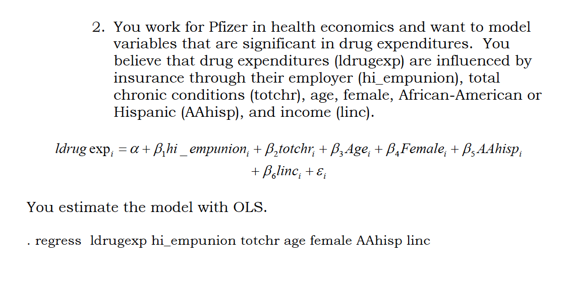
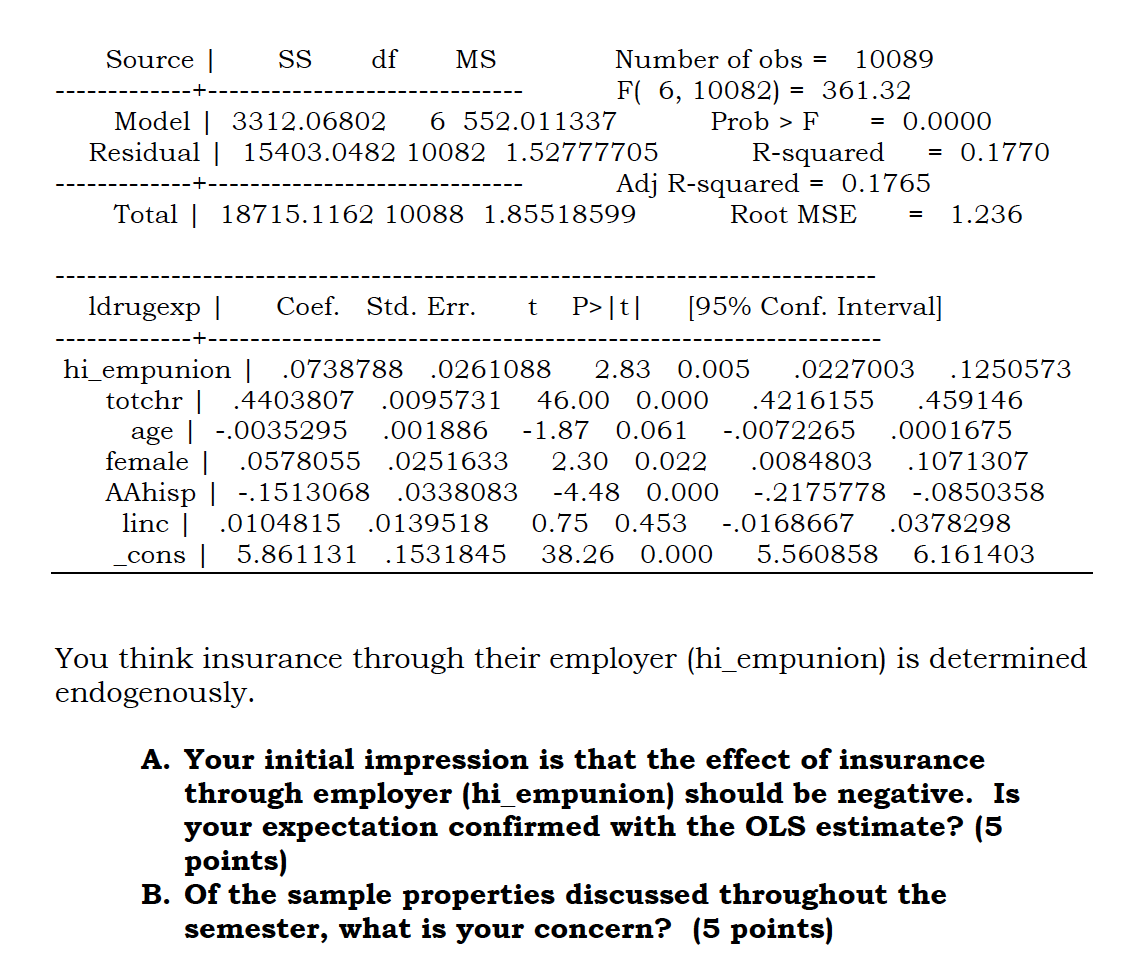
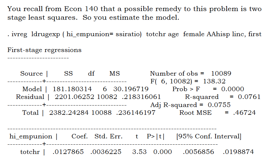
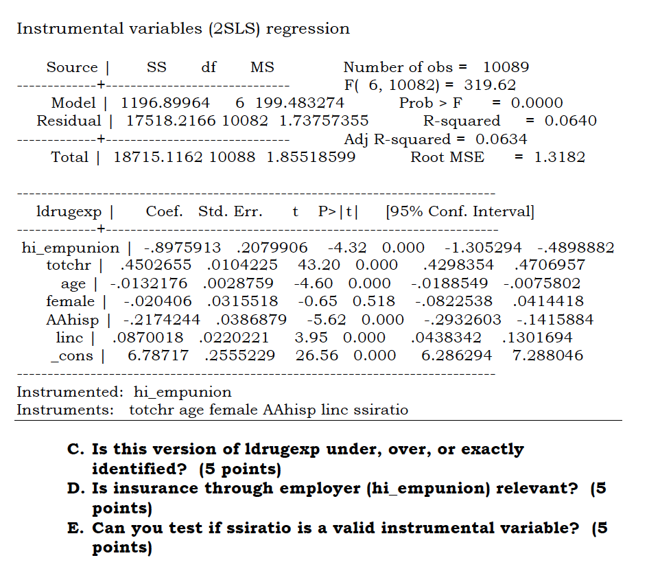
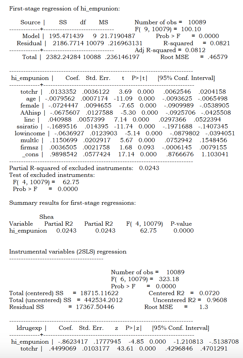
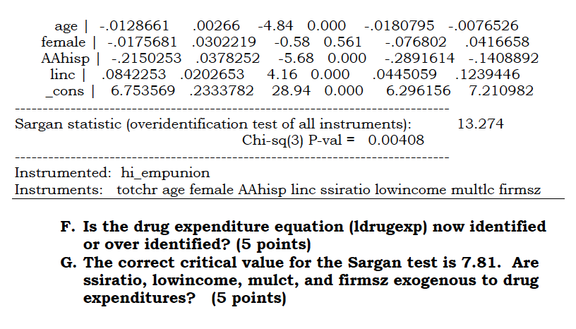
2. You work for Pfizer in health economics and want to model variables that are significant in drug expenditures. You believe that drug expenditures (ldrugexp) are influenced by insurance through their employer (hi_empunion), total chronic conditions (totchr), age, female, African-American or Hispanic (AAhisp), and income (linc). Idrug exp; = a + Bjhi_empunion; + B,totchr; + By Age; + BAFemale; + B, AAhisp; + Bolinc; + E; You estimate the model with OLS. . regress ldrugexp hi_empunion totchr age female AAhisp lincSource | SS df MS Number of obs = 10089 F( 6, 10082) = 361.32 Model | 3312.06802 6 552.011337 Prob > F = 0.0000 Residual | 15403.0482 10082 1.52777705 R-squared = 0.1770 Adj R-squared = 0.1765 Total | 18715.1162 10088 1.85518599 Root MSE 1.236 Idrugexp | Coef. Std. Err. t P> t| [95% Conf. Interval] hi_empunion | .0738788 .0261088 2.83 0.005 .0227003 . 1250573 totchr | .4403807 .0095731 46.00 0.000 .4216155 . 459146 age | -.0035295 .001886 -1.87 0.061 -.0072265 .0001675 female | .0578055 .0251633 2.30 0.022 .0084803 . 1071307 AAhisp | -.1513068 .0338083 -4.48 0.000 -.2175778 -.0850358 linc | .0104815 .0139518 0.75 0.453 -.0168667 0378298 cons 5.861131 .1531845 38.26 0.000 5.560858 6.161403 You think insurance through their employer (hi_empunion) is determined endogenously. A. Your initial impression is that the effect of insurance through employer (hi empunion) should be negative. Is your expectation confirmed with the OLS estimate? (5 points) B. Of the sample properties discussed throughout the semester, what is your concern? (5 points)You recall from Econ 140 that a possible remedy to this problem is two stage least squares. So you estimate the model. . ivreg ldrugexp ( hi_empunion= ssiratio) totchr age female AAhisp linc, first First-stage regressions Source SS df MS Number of obs = 10089 +- F( 6, 10082) = 138.32 Model | 181.180314 6 30.196719 Prob > F = 0.0000 Residual | 2201.06252 10082 .218316061 R-squared = 0.0761 Adj R-squared = 0.0755 Total | 2382.24284 10088 .236146197 Root MSE = .46724 hi_empunion | Coef. Std. Err. t P>|t| [95% Conf. Interval] totchr | .0127865 .0036225 3.53 0.000 .0056856 .0198874\fInstrumental variables (2SLS) regression Source | SS df MS Number of obs = 10089 F( 6, 10082) = 319.62 Model | 1196.89964 6 199.483274 Prob > F = 0.0000 Residual | 17518.2166 10082 1.73757355 R-squared = 0.0640 Adj R-squared = 0.0634 Total | 18715.1162 10088 1.85518599 Root MSE = 1.3182 Idrugexp | Coef. Std. Err. t P>|t| [95% Conf. Interval] + hi_empunion | -.8975913 .2079906 -4.32 0.000 -1.305294 -.4898882 totchr | .4502655 .0104225 43.20 0.000 .4298354 .4706957 age | -.0132176 .0028759 -4.60 0.000 -.0188549 -.0075802 female | -.020406 .0315518 -0.65 0.518 -.0822538 .0414418 AAhisp | -.2174244 .0386879 -5.62 0.000 -.2932603 -.1415884 linc | .0870018 .0220221 3.95 0.000 .0438342 . 1301694 _cons | 6.78717 .2555229 26.56 0.000 6.286294 7.288046 Instrumented: hi_empunion Instruments: totchr age female AAhisp linc ssiratio C. Is this version of ldrugexp under, over, or exactly identified? (5 points) D. Is insurance through employer (hi empunion) relevant? (5 points) E. Can you test if ssiratio is a valid instrumental variable? (5 points)Concerned that your IV cannot be tested, you nd additional variables that you think are related with insurance through employer {hi_empunion] but not related to the error. These variables are rm size {rmsz}, low income status (lowincome), and multiple locations (multlc). Firststage regressions First-stage regression of hi_empunion: Source | SS df MS Number of obs = 10089 F( 9, 10079) = 100.10 Model | 195.471439 9 21.7190487 Prob > F = 0.0000 Residual | 2186.7714 10079 .216963131 R-squared = 0.0821 Adj R-squared = 0.0812 Total | 2382.24284 10088 .236146197 Root MSE = .46579 hi_empunion | Coef. Std. Err. t P>|t| [95% Conf. Interval] totchr | .0133352 .0036122 3.69 0.000 .0062546 .0204158 age | -.0079562 .0007174 -11.09 0.000 -.0093625 -.0065498 female | -.0724447 .0094655 -7.65 0.000 -.0909989 -.0538905 AAhisp | -.0675607 .0127588 -5.30 0.000 -.0925706 -.0425508 linc | .040988 .0057399 7.14 0.000 .0297366 .0522394 ssiratio | -. 1689516 .014395 -11.74 0.000 -.1971688 -.1407345 lowincome | -.0636927 .0123903 -5.14 0.000 -.0879802 -.0394051 multlc | 1150699 .0202917 5.67 0.000 .0752942 . 1548456 firmsz | .0036505 .0021758 1.68 0.093 -.0006145 .0079155 cons .9898542 .0577424 17.14 0.000 .8766676 1. 103041 Partial R-squared of excluded instruments: 0.0243 Test of excluded instruments: F( 4, 10079) = 62.75 Prob > F = 0.0000 Summary results for first-stage regressions: Shea Variable Partial R2 Partial R2 F( 4, 10079) P-value hi_empunion 0.0243 0.0243 62.75 0.0000 Instrumental variables (2SLS) regression Number of obs = 10089 F( 6, 10079) = 323.18 Prob > F = 0.0000 Total (centered) SS = 18715.11622 Centered R2 = 0.0720 Total (uncentered) SS = 442534.2012 Uncentered R2 = 0.9608 Residual SS = 17367.50446 Root MSE 1.3 Idrugexp | Coef. Std. Err. z P>|z| [95% Conf. Interval] -+. hi_empunion | -.8623417 .1777945 -4.85 0.000 -1.210813 -.5138708 totchr | .4499069 .0103177 43.61 0.000 4296846 .4701291age | -.0128661 00266 -4.84 0.000 -.0180795 -.0076526 female | -.0175681 .0302219 -0.58 0.561 -.076802 .0416658 AAhisp | -.2150253 . .0378252 -5.68 0.000 -.2891614 -.1408892 linc | .0842253 .0202653 4.16 0.000 0445059 .1239446 _cons 6.753569 .2333782 28.94 0.000 6.296156 7.210982 Sargan statistic (overidentification test of all instruments): 13.274 Chi-sq(3) P-val = 0.00408 Instrumented: hi_empunion Instruments: totchr age female AAhisp linc ssiratio lowincome multlc firmsz F. Is the drug expenditure equation (ldrugexp) now identified or over identified? (5 points) G. The correct critical value for the Sargan test is 7.81. Are ssiratio, lowincome, mulct, and firmsz exogenous to drug expenditures? (5 points)