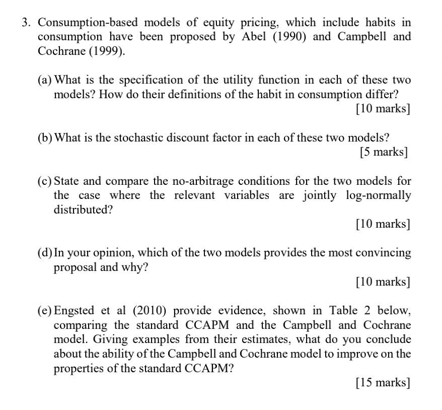
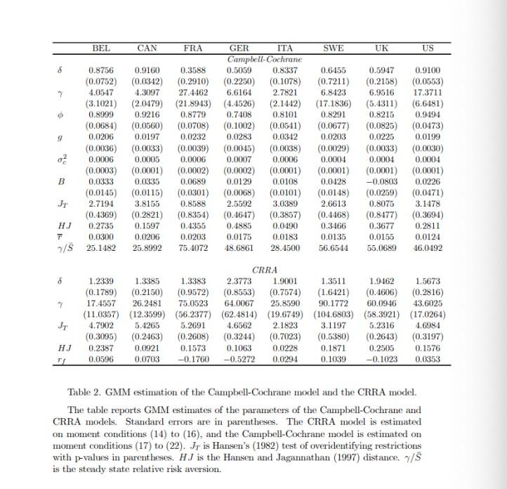
3. Consumption-based models of equity pricing, which include habits in consumption have been proposed by Abel (1990) and Campbell and Cochrane (1999). (a) What is the specification of the utility function in each of these two models? How do their definitions of the habit in consumption differ? [10 marks] (b) What is the stochastic discount factor in each of these two models? [5 marks] (c) State and compare the no-arbitrage conditions for the two models for the case where the relevant variables are jointly log-normally distributed? [10 marks] (d) In your opinion, which of the two models provides the most convincing proposal and why? [10 marks] (e) Engsted et al (2010) provide evidence, shown in Table 2 below, comparing the standard CCAPM and the Campbell and Cochrane model. Giving examples from their estimates, what do you conclude about the ability of the Campbell and Cochrane model to improve on the properties of the standard CCAPM? [15 marks] BEL CAN FRA GER ITA SWE UK US Campbell-Cochrane 0.8756 0.9160 0.3588 0.5059 0.8337 0.6455 0.5947 0.9100 (0.0752) (0.0342) (0.2910) (0.2250) (0.1078) (0.7211) (0.2158) (0.0553) 4.0547 4.3097 27.4462 6.6164 2.7821 6.8423 6.9516 17.3711 (3.1021) (2.0479) (21.8943) (4.4526) (2.1442) (17.1836) (5.4311) (6.6481) 0.8999 0.9216 0.8779 0.7408 0.8101 0.8291 0.8215 0.9494 (0.0684) (0.0560) (0.0708) (0.1002) (0.0541) (0.0677) (0.0825) (0.0473) 9 0.0206 0.0197 0.0232 0.0283 0.0342 0.0203 0.0225 0.0199 (0.0036) (0.0033) (0.0039) (0.0045) (0.0038) (0.0029) (0.0033) (0.0030) 0 0.0006 0.0005 0.0006 0.0007 0.0006 0.0004 0.0004 0.0004 (0.0003) (0.0001) (0.0002) (0.0002) (0.0001) (0.0001) (0.0001) (0.0001) B 0.0333 0.0335 0.0689 0.0129 0.0108 0.0428 -0.0803 0.0226 (0.0145) (0.0115) (0.0301) (0.0068) (0.0101) (0.0148) (0.0259) (0.0471) JT 2.7194 3.8155 0.8588 2.5592 3.0389 2.6613 0.8075 3.1478 (0.4369) (0.2821) (0.8354) (0.4647) (0.3857) (0.4468) (0.8477) (0.3694) HJ 0.2735 0.1597 0.4355 0.4885 0.0490 0.3466 0.3677 0.2811 T 0.0300 0.0206 0.0203 0.0175 0.0183 0.0135 0.0155 0.0124 7/8 25.1482 25.8992 75.4072 48.6861 28.4500 56.6544 55.0689 46.0492 CRRA 8 1.2339 1.3385 1.3383 2.3773 1.9001 1.5673 (0.1789) (0.2150) (0.9572) (0.8553) (0.7574) 1.3511 1.9462 (1.6421) (0.4606) (0.2816) 90.1772 60.0946 43.6025 7 17.4557 26.2481 75.0523 64.0067 25.8590 (11.0357) (12.3599) (56.2377) (62.4814) (19.6749) (104.6803) (58.3921) (17.0264) 4.7902 JT 5.2691 4.6562 2.1823 3.1197 5.2316 4.6984 (0.3095) 5.4265 (0.2463) (0.2608) 0.1573 (0.3244) (0.7023) 0.1063 0.0228 (0.5380) (0.2643) (0.3197) HJ 0.2387 0.0921 0.1871 0.2505 0.1576 0.0596 0.0703 -0.1760 -0.5272 0.0294 0.1039 -0.1023 0.0353 Table 2. GMM estimation of the Campbell-Cochrane model and the CRRA model. The table reports GMM estimates of the parameters of the Campbell-Cochrane and CRRA models. Standard errors are in parentheses. The CRRA model is estimated on moment conditions (14) to (16), and the Campbell-Cochrane model is estimated on moment conditions (17) to (22). Jr is Hansen's (1982) test of overidentifying restrictions with p-values in parentheses. HJ is the Hansen and Jagannathan (1997) distance. 7/5 is the steady state relative risk aversion. 6 7 3. Consumption-based models of equity pricing, which include habits in consumption have been proposed by Abel (1990) and Campbell and Cochrane (1999). (a) What is the specification of the utility function in each of these two models? How do their definitions of the habit in consumption differ? [10 marks] (b) What is the stochastic discount factor in each of these two models? [5 marks] (c) State and compare the no-arbitrage conditions for the two models for the case where the relevant variables are jointly log-normally distributed? [10 marks] (d) In your opinion, which of the two models provides the most convincing proposal and why? [10 marks] (e) Engsted et al (2010) provide evidence, shown in Table 2 below, comparing the standard CCAPM and the Campbell and Cochrane model. Giving examples from their estimates, what do you conclude about the ability of the Campbell and Cochrane model to improve on the properties of the standard CCAPM? [15 marks] BEL CAN FRA GER ITA SWE UK US Campbell-Cochrane 0.8756 0.9160 0.3588 0.5059 0.8337 0.6455 0.5947 0.9100 (0.0752) (0.0342) (0.2910) (0.2250) (0.1078) (0.7211) (0.2158) (0.0553) 4.0547 4.3097 27.4462 6.6164 2.7821 6.8423 6.9516 17.3711 (3.1021) (2.0479) (21.8943) (4.4526) (2.1442) (17.1836) (5.4311) (6.6481) 0.8999 0.9216 0.8779 0.7408 0.8101 0.8291 0.8215 0.9494 (0.0684) (0.0560) (0.0708) (0.1002) (0.0541) (0.0677) (0.0825) (0.0473) 9 0.0206 0.0197 0.0232 0.0283 0.0342 0.0203 0.0225 0.0199 (0.0036) (0.0033) (0.0039) (0.0045) (0.0038) (0.0029) (0.0033) (0.0030) 0 0.0006 0.0005 0.0006 0.0007 0.0006 0.0004 0.0004 0.0004 (0.0003) (0.0001) (0.0002) (0.0002) (0.0001) (0.0001) (0.0001) (0.0001) B 0.0333 0.0335 0.0689 0.0129 0.0108 0.0428 -0.0803 0.0226 (0.0145) (0.0115) (0.0301) (0.0068) (0.0101) (0.0148) (0.0259) (0.0471) JT 2.7194 3.8155 0.8588 2.5592 3.0389 2.6613 0.8075 3.1478 (0.4369) (0.2821) (0.8354) (0.4647) (0.3857) (0.4468) (0.8477) (0.3694) HJ 0.2735 0.1597 0.4355 0.4885 0.0490 0.3466 0.3677 0.2811 T 0.0300 0.0206 0.0203 0.0175 0.0183 0.0135 0.0155 0.0124 7/8 25.1482 25.8992 75.4072 48.6861 28.4500 56.6544 55.0689 46.0492 CRRA 8 1.2339 1.3385 1.3383 2.3773 1.9001 1.5673 (0.1789) (0.2150) (0.9572) (0.8553) (0.7574) 1.3511 1.9462 (1.6421) (0.4606) (0.2816) 90.1772 60.0946 43.6025 7 17.4557 26.2481 75.0523 64.0067 25.8590 (11.0357) (12.3599) (56.2377) (62.4814) (19.6749) (104.6803) (58.3921) (17.0264) 4.7902 JT 5.2691 4.6562 2.1823 3.1197 5.2316 4.6984 (0.3095) 5.4265 (0.2463) (0.2608) 0.1573 (0.3244) (0.7023) 0.1063 0.0228 (0.5380) (0.2643) (0.3197) HJ 0.2387 0.0921 0.1871 0.2505 0.1576 0.0596 0.0703 -0.1760 -0.5272 0.0294 0.1039 -0.1023 0.0353 Table 2. GMM estimation of the Campbell-Cochrane model and the CRRA model. The table reports GMM estimates of the parameters of the Campbell-Cochrane and CRRA models. Standard errors are in parentheses. The CRRA model is estimated on moment conditions (14) to (16), and the Campbell-Cochrane model is estimated on moment conditions (17) to (22). Jr is Hansen's (1982) test of overidentifying restrictions with p-values in parentheses. HJ is the Hansen and Jagannathan (1997) distance. 7/5 is the steady state relative risk aversion. 6 7