3 In 0900'0 500O'D 1000 0 FIG. 4. Process H alloy composition: (a) & chart, (b) "chart based on log ratios, (o) X' versus 73. S 0900'0 50COD 100070 S602 R. A. Boyles For this data set, step (3) in Section 4.2 yields = 4 after rounding up to the nearest integer. Figure 5 shows the X chart (Fig. 5(a)), the * chart based on log- ratio data analogous to equation (16) (Fig. 5(b)) and the scatterplot of X by T (Fig. 5(c)). The performance of X relative to T' is similar to that observed in the particle size distribution case study in Section 5.1, with 7 identifying two out-of- control points not detected by X , and X identifying one point not detected by T . This data set shows signs of autocorrelation between successive daily checks. This is especially evident in Fig. 5 (a). At present, there are no control charting techniques for multivariate auto correlated data. This is an important area for further search. Such methods will inevitably require more sophisticated computational environ- ments than methods for the independent identically distributed case. Given this, there is no reason why they could not be used for shopfloor process monitoring. 7 Summary and conclusions We have developed a modified chi-square control chart that is suitable for shopfloor monitoring of compositional process data. The two main advantages of this technique are that it requires only basic arithmetic operations and statistical functions (mean and variance), and that many technical staff will be familiar with the chi-square test from their basic statistical training. The disadvantage is that it can be less sensitive than the 7 chart. We have found in case studies that this is not a major practical problem, especially in the first stages of statistical monitoring when easily detected assignable causes are relatively plentiful. In our case studies, the availability of a simple multivariate method was the key factor in management decisions to go ahead with shopfloor statistical monitoring programs, which have since proven themselves as value-adding activities. Acknowledgements The author thanks his colleague Donal Krouse for reading preliminary versions of this report and making suggestions that led to significant improvements in the content and presentation. Thanks also to Precision Castparts Corp., for providing the data sets in Sections 5.1, 5.2 and 6.2, and to BHP New Zealand Steel Lid, for providing the data set in Section 6.1. REFERENCES AITCHISON, J. (1946) The Sunsical Analysis of Compositional Dam (London, Chapman and Hall). ANDERSON, T. W. (1954) An Introduction to Mulavariare Statistical Analysis (New York, Wiley). DUNCAN, A. J. (1950) A chi-square chart for controlling a set of percentages, Indunrial Quality Comral, 7, pp. 11-15. HOLMES, D. S. & ZOOK, R. D. (1990) Using chi-square and T-square charts to interpret sieve analysis data, Ponder and Bulk Engineering, February, pp. 30-36.Let x= (x1,x3....x) have the multinomial distribution .(n, 10), where It= (misty.,*;) is a vector of positive probabilities that sum to 1. The probability mass function is PO)= *! .. XA! for non-negative integer-valued x,, with ait ant .. .+ %,= n. Let u= x/m. Then E(u) = n and Cov (u) = {Ding (n) - n}/ As #->0, u has an asymptotic multivariate normal distribution with mean It and the (singular) covariance given above. Let y and of be defined by V = 1/2 (3) and p= (x1 . . .3* ) (4) Then, E(v) = 0 and Cov(v) = (1 - pp) (5) As #->0, v has an asumptotic multivariate normal distribution with mean 0 and the (singular) covariance of equation (5). Note that vv coincides with X" in equation (2), and that avv is the usual chi- square statistic, i.e. HV V= # Note that bob= 1, and let the columns of the AX & (1 - 1) matrix A comprise the remainder of an orthonormal basis. Then, we have A'A = I-15 AA'= 1,- q (6) Let w = A v. Then, from equations (5) and (6), we have Cov (w) = A'(I, - (()A/ = 1-1/ Because cv= 0, equation (6) also impliesNote that pop= 1, and let the columns of the AX & ()- 1) matrix A comprise the remainder of an orthonormal basis. Then, we have AA= I-1, AA'= 1,- (p' (6) Let w = A v. Then, from equations (5) and (6), we have Cov (w) = A'I, - (6)A/= 1 1/ Because cv= 0, equation (6) also implies ww =v'(I-

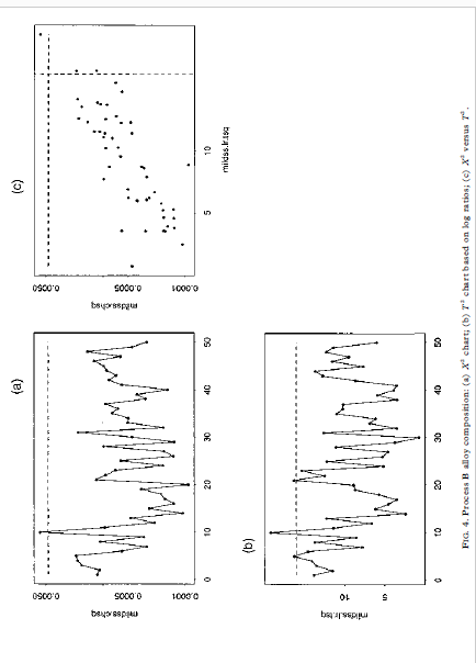
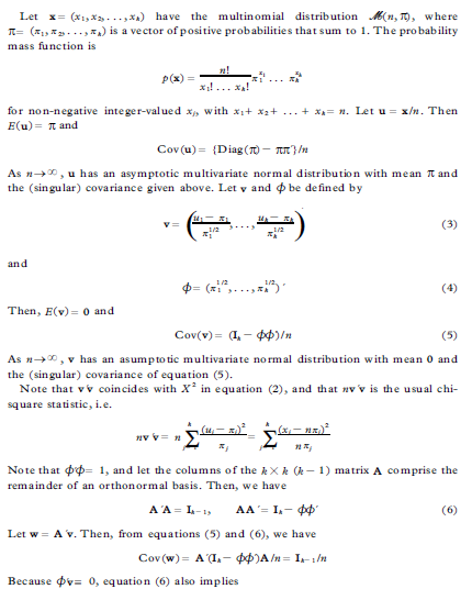
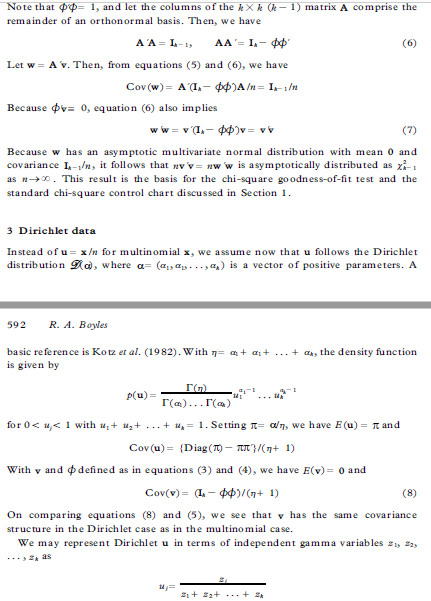
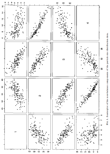
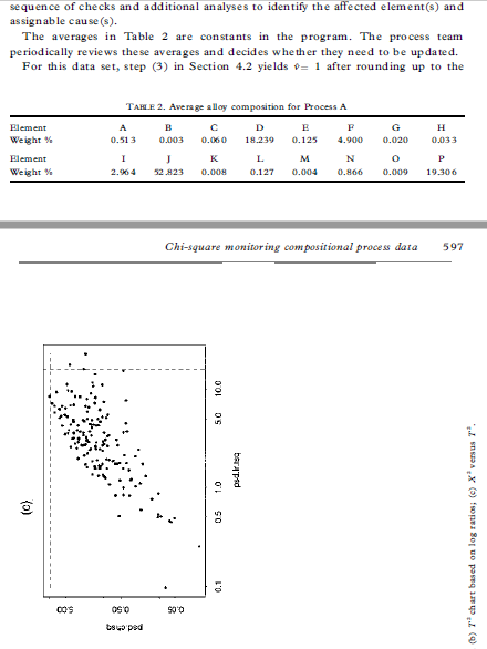
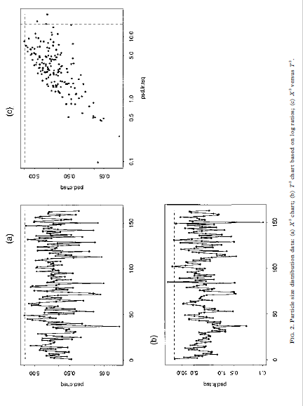
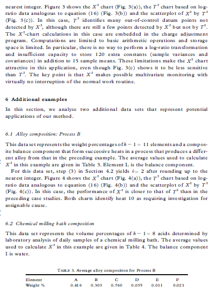
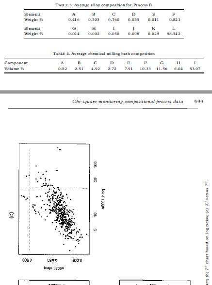
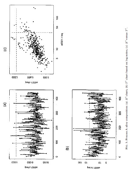
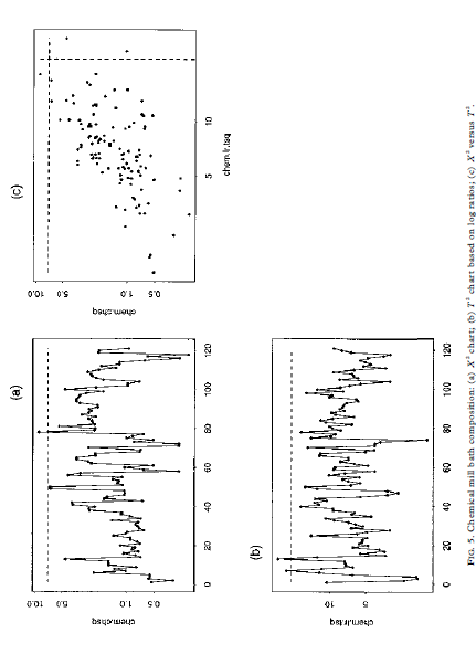
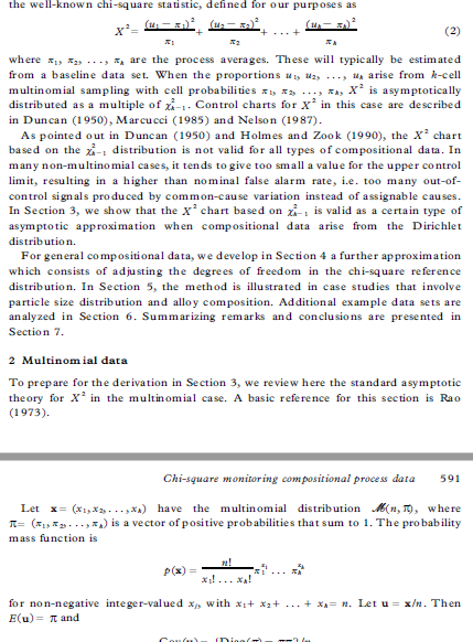
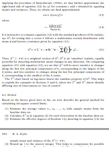
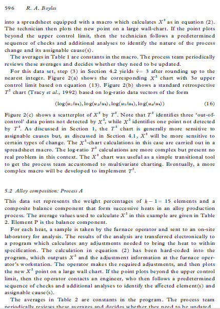
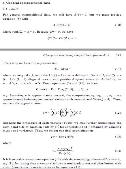
00, the vectors u and v are asymptotically muluvariate normal as 700 for fixed It. By the argument given in Section 2, (7+ 1)vv is asymptotically distributed as zi-, as q 00 for fixed It This approximation entails E(vv)= ()-1)/(q+ 1) from which we obtain the distributional approximation in its most useful form, i.e. vVx E(vv)ni/(4-1) (9) Note the analogy between equation (9) and the normal-theory distribution of the sample variance, i.e. geox/(- 1) where a = E(s ). Using this analogy, the easiest way to implement a control chart based on equation (9) is to use the X' values as input to a standard S' chart of sample variances (Montgomery, 1991), where & is used as the sample size. Here, one would suppress the lower control limit and set the upper control limit to give the overall '3a" false alarm rate of 0.0027. 4 General compositional data 4.1 Theory For general compositional data, we still have E(v) = 0, but we must replace equation (8) with Cov(v) = E (10) where rank (2) = # - 1. Because cv= 0, we have DE= Var(pv) = 0 Chi-square monitoring compositional process data 5934.2 Method Based on the theory given here so far, we now describe the general method for calculating chi-square control limits. (1) Estimate the average values x1, zay ..., x, with sample means from the baseline data set. (2) Calculate X as in equation (2) for each observation in the baseline data set. (3) Estimate the effective degrees of freedom + by inserting in equation (14) the 594 R. A. Boyles sample mean and variance of the X (= vv). (4) Round up + to the nearest integer. This helps to compensate for possible variance-inflating effects of 'out-of-control' X" points, although + seems to be relatively insensitive to these. (5) Calculate the upper control limit by inputing the X data to a standard 5" charting procedure, using v+ 1 as the sample size. The upper limit should be set to give the overall '3a" false alarm rate of 0.0027. The lower control limit should be suppressed. (6) Follow standard charting procedure for removing extreme outliers (high X] values) and recalculating the upper control limit within the S charting procedure. Usually, it is not necessary to go back to step (1) to recalculate the X values and v. 5 Case studies In this section, we discuss two case studies that involve the method proposed here. In each case, a multivariate chart was the key to shopfloor monitoring of compositional process data. The key factors in 'selling" the chi-square chart were the simplicity of the X calculation in equation (2), and the familiarity of technical staff with the chi-square goodness-of-fit test, as obtained from their basic statistical training. In these examples, shopfloor monitoring led to process improvements, including the discovery and resolution of measurement problems; reductions in unplanned equipment downtime; the discovery and resolution of raw materials problems; improvements in operating procedures; and improvements in the quality of products downstream. For each example, we analyze here the baseline data set used to initiate statistical monitoring.5 Case studies In this section, we discuss two case studies that involve the method proposed here. In each case, a multivariate chart was the key to shopfloor monitoring of compositional process data. The key factors in 'selling" the chi-square chart were the simplicity of the X calculation in equation (2), and the familiarity of technical staff with the chi-square goodness-of-fit test, as obtained from their basic statistical training. In these examples, shopfloor monitoring led to process improvements, including the discovery and resolution of measurement problems; reductions in unplanned equipment downtime; the discovery and resolution of raw materials problems; improvements in operating procedures; and improvements in the quality of products downstream. For each example, we analyze here the baseline data set used to initiate statistical monitoring. 5.1 Particle size distribution This data set represents daily checks on the particle size distribution of a ceramic stucco used to make shells for investment casting. There are *= 5 particle size ranges, with range 5 being a balance component calculated as 100 minus the sum of the other four ranges. The average values used to calculate X in this example are given in Table 1. Figure 1 shows scatterplots of ranges 1-4. Note that range 1 is positively correlated with range 2, and range 3 is positively correlated with range 4. These positive correlations violate the multinomial/Dirichlet correlation structure reflected in equations (5) and (8). Positive correlations are common in composi- tional process data, indicating the need for models that are more flexible than the Dirichlet approach (Aitchison, 1986). In the present context, non-Dirichlet correlation structures are the reason for the degrees-of-freedom adjustment developed in Section 4.1. For each daily check, a technician extracts a sample of the stucco, performs a sieve analysis (see Holmes & Zook, 1990), and then enters the weight percentages TABLE 1. Average particle size distribution Size range 1 2 3 5 Weight 4.24 55.80 29.00 0.85 1.05 Chi-square monitoring compositional process data 5952. FIG. 1. Scatterplot of the non-balance components of the particle abe distribution data. 5 09 S+sequence of checks and additional analyses to identify the affected element(s) and assignable cause (s). The averages in Table 2 are constants in the program. The process team periodically reviews these averages and decides whether they need to be updated. For this data set, step (3) in Section 4.2 yields = 1 after rounding up to the TAH E 2. Average alloy composition for Process A Element A C D G H Weight 0.513 0.010 14.239 0.125 4.900 0.020 Element K L. M N Weight : 2.964 52.423 O. OOH 0.127 0.004 19.300 Chi-square monitoring compositional process data 597 50 10 0 05 (b) T' chart based on log ration; (o) X' versus Ta 0S'O 90 0CO'S 08'0 90 0 100 05 50 100 batyped 0'1 0 100 150 FIG. 2. Particle size distribution data: (a) X" chart, (b) T' chart based on log ratios, (o) X'' versus 7.nearest integer. Figure 3 shows the X' chart (Fig. 3(a)), the 7 chart based on log- ratio data analogous to equation (16) (Fig. 3(b)) and the scatterplot of X by T (Fig. 3(c)). In this case, T identifies many out-of-control datum points not detected by X , although there are still a few points detected by X but not by T. The X'-chart calculations in this case are embedded in the charge adjustment program. Computations are limited to basic arithmetic operations and storage space is limited. In particular, there is no way to perform a log-ratio transformation and insufficient capacity to store 120 extra constants (sample variances and covariances) in addition to 15 sample means. These limitations make the X chart attractive in this application, even though Fig. 3(c) shows it to be less sensitive than 7 . The key point is that X' makes possible multivariate monitoring with virtually no interruption of the normal work routine. 6 Additional examples In this section, we analyze two additional data sets that represent potential applications of our method. 6.1 Alloy composition: Process B This data set represents the weight percentages of - 1 = 11 elementsand a compos- ite balance component that form successive heats in a process that produces a differ- ent alloy from that in the preceding example. The average values used to calculate X in this example are given in Table 3. Element L is the balance component. For this data set, step (3) in Section 4.2 yields = 2 after rounding up to the nearest integer. Figure 4 shows the X chart (Fig. 4(a)), the 7 chart based on log- ratio data analogous to equation (16) (Fig. 4(b)) and the scatterplot of X by T (Fig. 4(c)). In this case, the performance of X is closer to that of 7 than in the preceding case studies. Both charts identify heat 10 as requiring investigation for assignable cause. 6.2 Chemical milling bath composition This data set represents the volume percentages of k- 1= 8 acids determined by laboratory analysis of daily samples of a chemical milling bath. The average values used to calculate X in this example are given in Table 4. The balance component I is water. TAKE 3. Average alloy composition for Process B Plement A C D F Weight %% 0.416 0.303 0.760 0.035 0.011 0.021TAKE 3. Average alloy composition for Process B Element A H C Weight " 0.416 0.309 0.760 0.035 0.011 0702 1 Plement G H K Weight 0.02 4 0.002 0.050 0.OOH 0.029 94.342 TABLE 4. Average chemical milling bath composition Component A B C D F G H Volume Vi 0.02 2.51 4.92 2.72 7.91 10.33 11.56 6.04 53.07 Chi-square monitoring compositional process data 599 100 46021.hbaq art (b) T' chart based on log ratios; (c) X' versus 7. 080'0 910'0 4602 1. chiq060'0 05010 910'0 100 200 100 400 100 46021.hisq 001 01 but 18090 S 100 200 300 400 FIG. 3. Process A alloy composition: (a) X" chart (b) " chart based on log ratios; (c) X' versus T).Using the chi-square statistic to monitor compositional process data RUSSELL A. BOYLES, New Zealand Institute of Industrial Research and Develop- ment, Lower Hunt, New Zealand SUMMARY We investigate the use of the chi-square control chart as a simple multi variate method for shopfloor monitoring of compositional process data. Although this chart is usually considered to be applicable only with muhinomial process data, we show that it is also valid, in a certain asymptotic sense, for compositional data that arise from the Dirichler distribution. For general compositional data, we show that the chi-square staristic can be used for process monitoring, provided that we make a simple adjustment to the degrees of freedom in the chi-square reference distribution. This method is illustrated and compared in four examples with the T' chart based on log-ratio transformation of the data. 1 Introduction Compositional data are measurements My ty .... #, where & is the number of components, a, is the proportion associated with the ith component and w+ met .. . + = 1 (1) Compositional data are often expressed as percentages rather than as proportions, in which case, the right-hand side of equation (1) would be 100 rather than 1. In many real compositional data sets, the fundamental property in equation (1) is compromised through the effects of measurement error. In many cases, this problem is handled by treating one of My My .... " as a 'balance' component which is redefined so that equation (1) holds exactly. Compositional data are frequently encountered in the chemical and process industries. Common examples involve products or process materials that are chemical mixtures of several ingredients. Aitchison (1986) gives 40 compositional data sets that represent a wide range of industrial and scientific applications. Thewhich is redefined so that equation (1) holds exactly. Compositional data are frequently encountered in the chemical and process industries. Common examples involve products or process materials that are chemical mixtures of several ingredients. Aitchison (1986) gives 40 compositional data sets that represent a wide range of industrial and scientific applications. The examples discussed in this paper represent three types of compositional data: Comespendence: R. A. Boyles, 3099 Rosemary Lane, Lake Oswego, OR 97034, USA. 0266-4763/97/050589-14 57.00 #1997 Carfax Publishing Lid 590 R. A. Boyles particle size distribution, where each component is a size range; alloy composition, where each component is an element or combination of elements; and chemical milling bath composition, where one component is water and the others are acids. The measurements are weight percentages in the first two cases and volume percentages in the third case. The methodology presented applies to any type of compositional data used for process monitoring. For statistically monitoring compositional data, a sensible approach would be to apply the log-ratio transformation described in Aitchison (1986) and to monitor the resulting () - 1)-dimensional data vectors with a standard 7' chart for individual observations (Tracy er al., 1992). As described in Anderson (1958, Section 5.5) and other multivariate analysis texts, " is uniformly the most powerful among a broad class of statistics for detecting unanticipated changes in a multivariate mean. In the control charting context, this means that the 7 chart has the greatest probability of detecting assignable causes. Even today, the computational complexity of the optimal approach described above makes it impractical in many shopfloor situations. However, in shopfloor situations that involve complex processes, a multivariate approach is appealing, because it can dramatically reduce the number of charts that require operator monitoring. This is convenient from a practical point of view, and also provides better control of the overall false alarm rate (type I error). In this paper, we investigate a less powerful but more easily implemented multivariate procedure. We propose monitoring compositional process data with the well-known chi-square statistic, defined for our purposes as (2) where ais to .. ., a, are the process averages. These will typically be estimated from a baseline data set. When the proportions My Way .... in arise from k-cell multinomial sampling with cell probabilities ay ay .... an, A is asymptotically distributed as a multiple of _ Control charts for X' in this case are describedcham. I.teq It (b) "' chart based on log radios; (o) X' versus Ti D'OR O'S SO 120 120 100 100 2 2 D'L 90the well-known chi-square statistic, defined for our purposes as + (2) where an ty ..., I, are the process averages. These will typically be estimated from a baseline data set. When the proportions My way .... " arise from A-cell multinomial sampling with cell probabilities zy zy ..., xx, X is asymptotically distributed as a multiple of zi-1. Control charts for X in this case are described in Duncan (1950), Marcucci (1985) and Nelson (1987). As pointed out in Duncan (1950) and Holmes and Zook (1990), the X chart based on the z-, distribution is not valid for all types of compositional data. In many non-multinomial cases, it tends to give too small a value for the upper control limit, resulting in a higher than nominal false alarm rate, i.e. too many out-of- control signals produced by common-cause variation instead of assignable causes. In Section 3, we show that the X chart based on zi , is valid as a certain type of asymptotic approximation when compositional data arise from the Dirichlet distribution. For general compositional data, we develop in Section 4 a further approximation which consists of adjusting the degrees of freedom in the chi-square reference distribution. In Section 5, the method is illustrated in case studies that involve particle size distribution and alloy composition. Additional example data sets are analyzed in Section 6. Summarizing remarks and conclusions are presented in Section 7. 2 Multinomial data To prepare for the derivation in Section 3, we review here the standard asymptotic theory for X in the multinomial case. A basic reference for this section is Rao (1973). Chi-square monitoring compositional process data 591 Let x= (x1,x3 . ..,* ) have the multinomial distribution .(n, 10), where I= (* *y . ..,* ) is a vector of positive probabilities that sum to 1. The probability mass function is P() = "I .. XI! . . . XA! for non-negative integer-valued x, with xit xit ... + %,= n. Let u = x/m. Then E(u) = n andApplying the procedure of Satterthwaite (1946), we may further approximate the right-hand side of equation (12) by cy, for constants c and v obtained by equating means and variances. Thus, we obtain our final approximation VV E(vv);/v (13) where V= (14) Var(v v) It is instructive to compare equation (12) with the standard goodness-of-fit statistic, say G', for testing that a vector v follows a multivariate normal distribution with mean o and known covariance given by equation (11): G'=VIV= WD W= E (15) Thus, X (= vv) is a weighted version of G'. G' is an 'omnibus' statistic, equally powerful for detecting multivariate mean changes in any direction. On comparing equation (15) with equation (12), we see that X will be more sensitive to changes along the first few principal components of v, corresponding to the largest of the 6 terms, and less sensitive to changes along the last few principal components of v, corresponding to the smallest of the 5, terms. The T' chart based on log-ratios shares the omnibus property of G . This helps to explain the examples in Sections 5 and 6, where the 7 and X charts identify differing sets of observations as 'out of control'. 4.2 Method Based on the theory given here so far, we now describe the general method for calculating chi-square control limits. (1) Estimate the average values x1, za, .... NA with sample means from the baseline data set. (2) Calculate X as in equation (2) for each observation in the baseline data set. (3) Estimate the effective degrees of freedom by inserting in equation (14) the 594 R. A. Boyles sample mean and variance of the X (= vv). (4) Round up & to the nearest integer. This helps to compensate for possible596 R. A. Boyles into a spreadsheet equipped with a macro which calculates Xas in equation (2). The technician then plots the new point on a large wall-chart. If the point plots beyond the upper control limit, then the technician follows a predetermined sequence of checks and additional analyses to identify the nature of the process change and its assignable cause(s). The averages in Table 1 are constants in the macro. The process team periodically reviews these averages and decides whether they need to be updated. For this data set, step (3) in Section 4.2 yields *= 3 after rounding up to the nearest integer. Figure 2(a) shows the corresponding X chart with 30 upper control limit based on equation (13). Figure 2(b) shows a standard retrospective I' chart (Tracy er al., 1992) based on log-ratio data vectors of the form (log (m/us), log(w/us), log(my/us), log( name)) (16) Figure 2(c) shows a scatterplot of X" by 7 . Note that T identifies three 'out-of- control' data points not detected by X , while X identifies one point not detected by 7 . As discussed in Section 1, the T' chart is generally more sensitive to assignable causes but, as discussed in Section 4.1, X' will be more sensitive to certain types of change. The X-chart calculations in this case are carried out in a spreadsheet macro. The log-ratio 7 calculations are more complex but present no real problem in this context. The X chart was useful as a simple transitional tool to get the process team accustomed to multivariate charting. Eventually, a more complex macro will be developed to implement 7 . 5.2 Alloy composition: Process A This data set represents the weight percentages of A- 1= 15 elements and a composite balance component that form successive heats in an alloy production process. The average values used to calculate X" in this example are given in Table 2. Element P is the balance component. For each heat, a sample is taken by the furnace operator and sent to an on-site laboratory for analysis. The results of the analysis are transferred electronically to a program which calculates any adjustments needed to bring the heat to within specification. The calculation in equation (2) has been hard-coded into the program, which outputs X and the adjustment information at the furnace oper- ator's workstation. The operator makes the required adjustments, and then plots the new X point on a large wall chart. If the point plots beyond the upper control limit, then the operator contacts an engineer, who then follows a predetermined sequence of checks and additional analyses to identify the affected element(s) and assignable cause (s). The averages in Table 2 are constants in the program. The process team periodically reviews these averaces and decides whether they need in he undated4 General compositional data 4.1 Theory For general compositional data, we still have E(v) = 0, but we must replace equation (8) with Cov(v) = _ (10) where rank (E) = 4 - 1. Because pv= 0, we have pro= Var(bv) = 0 Chi-square monitoring compositional process data 593 Therefore, we have the representation E= ADA' (1 1) where we may take A to be the 4 X (4 - 1) matrix defined in Section 2, and D is a (k - 1) X () - 1) diagonal matrix with positive diagonal elements. As before, let w = Av, so that vv= ww. From equations (6) and (11), we have Cov (w) = D = Diag (61, 8;,. .., 61.) say. Assuming v is approximately normal, the components Wi, Wa, . ... -1 are approximately independent normal variates with mean 0 and Var(w,) = 6, . Thus, we have the approximation V V= (12) Applying the procedure of Satterthwaite (1946), we may further approximate the right-hand side of equation (12) by cy, for constants c and v obtained by equating means and variances. Thus, we obtain our final approximation VV~ E(vV)x/v (13) where V = (14) Var(v v) It is instructive to compare equation (12) with the standard goodness-of-fit statistic, say G', for testing that a vector v follows a multivariate normal distribution with mean o and known covariance given by equation (11)