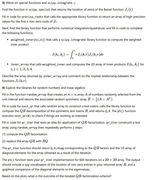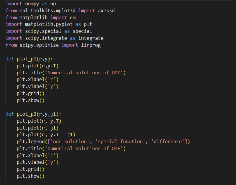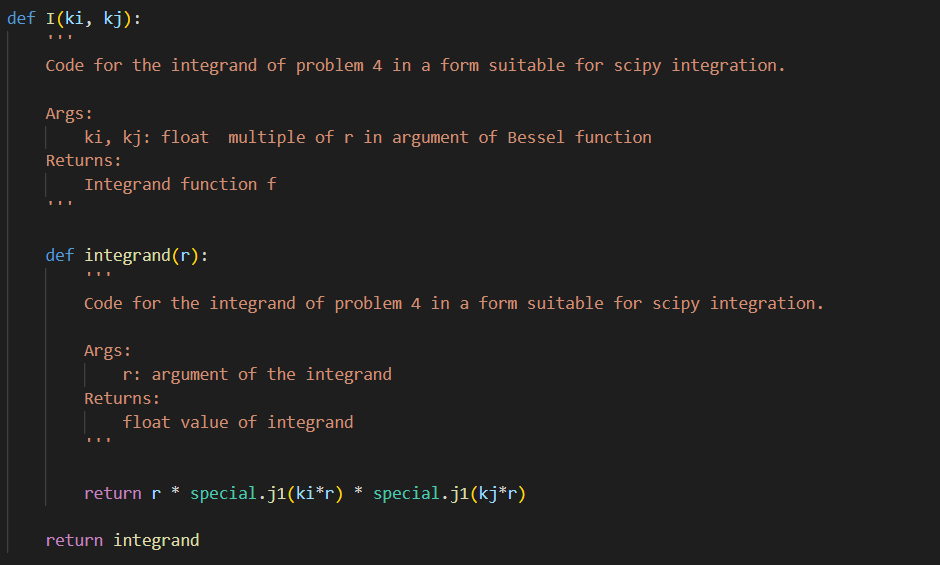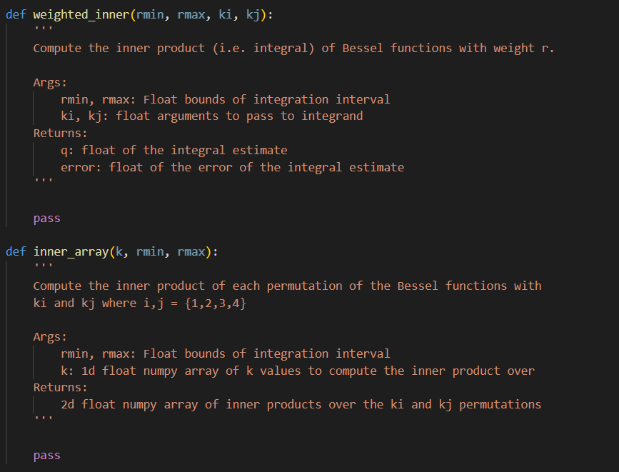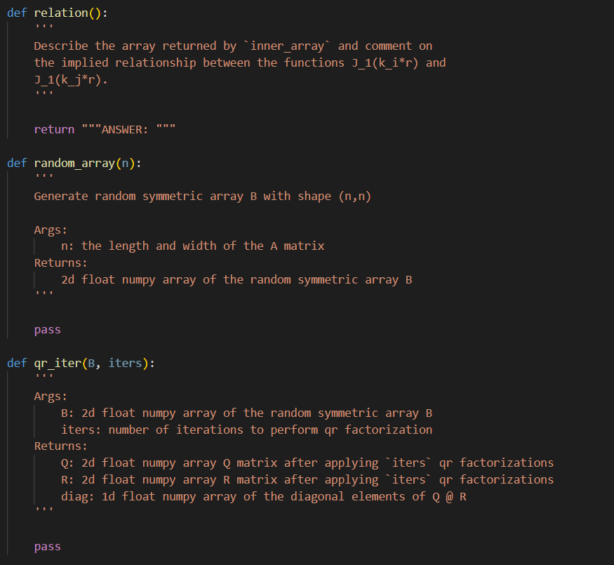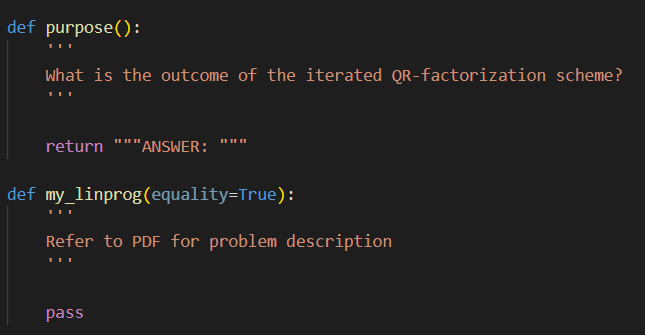
3) (More on special functions and scipy. integrate...) Find the function in scipy. special that returns the location of zeros of the Bessel function J1(r). Fill in code for precise_roots that calls the appropriate library function to return an array of high-precision values for the first n non-zero roots of J1. Next, find the library function that performs numerical integration/quadrature, and fill in code to complete the following functions: - weighted_inner (ki,kj) that calls a scipy. integrate library function to compute the weighted inner product I(ki,kj)=01rJ1(kir)J1(kjr)dr - inner_array that calls weighted_inner and computes the 2D array of inner products I(ki,kj) for i,j1,2,3,4 Describe the array returned by inner_array and comment on the implied relationship between the functions J1(kir). 4) Explore the libraries for random numbers and linear algebra. Fill in the function random_array that creates an nn array A of numbers randomly selected from the unit interval and returns the associated random symmetric array B=21(A+AT). Fill in code for test_qr that calls random array to construct a test matrix, calls the library function to compute the QR decomposition of the symmetric test matrix B, and returns Q,R. The p5 () function executes test_qr(8) to check if things are working as intended. Fill in code for qr_iter that tests an idea for application of QR-factorization. qr_iter constructs a test array using random_array then repeatedly performs 2 steps: (1) compute the QR factorization. (2) replace the array QR with RQ. The qr_iter function should return Q,R, diag corresponding to the QR factors and the 1D array of diagonal elements for the array obtained as a result of the iteration. The p5() function tests your qr_iter implementation for 600 iterations on a 2020 array. The output should include a spy visualization of the location of non-zero entries in your returned array R, and a graphical comparison of the diagonal elements to the eigenvalues. Based on the plots, what is the outcome of the iterated QR-factorization scheme? import numpy as np from mpl_toolkits.mplot3d import axes 3 d from matplotlib import cm import matplotlib.pyplot as plt import scipy.special as special import scipy.integrate as integrate from scipy.optimize import linprog def plot_p1(r,y): plt.plot(r,y.T) plt.title('Numerical solutions of oDE') plt.xlabel('r') plt.ylabel('y') plt.grid() plt.show() def plot_p2(r,y,j1): plt.plot(r,y.T) plt.plot(r, j1) plt.plot(r, r.T - j1) plt.legend(['ode solution', 'special function', 'difference']) plt.title('Numerical solutions of oDE') plt.xlabel('r') plt.ylabel('y') plt.grid() plt. show() def precise_roots (n) : Find and evaluate the library function to determine where the zeros of a bessel function J_ 1 reside. Args: n: the number of desired roots for the bessel function J_1 Returns: 1D float numpy array of floats specifiying the zero locations pass I (ki,kj) : Code for the integrand of problem 4 in a form suitable for scipy integration. Args: Ri, kj: float multiple of r in argument of Bessel function Returns: def integrand function f Code for the integrand of problem 4 in a form suitable for scipy integration. Args: r : argument of the integrand Returns: float value of integrand return r * special.j1(ki*r) special.j1(kj*r) return integrand def purpose(): What is the outcome of the iterated QR-factorization scheme? return "'ANSWER: "'" def my_linprog(equality=True): Refer to PDF for problem description "' 3) (More on special functions and scipy. integrate...) Find the function in scipy. special that returns the location of zeros of the Bessel function J1(r). Fill in code for precise_roots that calls the appropriate library function to return an array of high-precision values for the first n non-zero roots of J1. Next, find the library function that performs numerical integration/quadrature, and fill in code to complete the following functions: - weighted_inner (ki,kj) that calls a scipy. integrate library function to compute the weighted inner product I(ki,kj)=01rJ1(kir)J1(kjr)dr - inner_array that calls weighted_inner and computes the 2D array of inner products I(ki,kj) for i,j1,2,3,4 Describe the array returned by inner_array and comment on the implied relationship between the functions J1(kir). 4) Explore the libraries for random numbers and linear algebra. Fill in the function random_array that creates an nn array A of numbers randomly selected from the unit interval and returns the associated random symmetric array B=21(A+AT). Fill in code for test_qr that calls random array to construct a test matrix, calls the library function to compute the QR decomposition of the symmetric test matrix B, and returns Q,R. The p5 () function executes test_qr(8) to check if things are working as intended. Fill in code for qr_iter that tests an idea for application of QR-factorization. qr_iter constructs a test array using random_array then repeatedly performs 2 steps: (1) compute the QR factorization. (2) replace the array QR with RQ. The qr_iter function should return Q,R, diag corresponding to the QR factors and the 1D array of diagonal elements for the array obtained as a result of the iteration. The p5() function tests your qr_iter implementation for 600 iterations on a 2020 array. The output should include a spy visualization of the location of non-zero entries in your returned array R, and a graphical comparison of the diagonal elements to the eigenvalues. Based on the plots, what is the outcome of the iterated QR-factorization scheme? import numpy as np from mpl_toolkits.mplot3d import axes 3 d from matplotlib import cm import matplotlib.pyplot as plt import scipy.special as special import scipy.integrate as integrate from scipy.optimize import linprog def plot_p1(r,y): plt.plot(r,y.T) plt.title('Numerical solutions of oDE') plt.xlabel('r') plt.ylabel('y') plt.grid() plt.show() def plot_p2(r,y,j1): plt.plot(r,y.T) plt.plot(r, j1) plt.plot(r, r.T - j1) plt.legend(['ode solution', 'special function', 'difference']) plt.title('Numerical solutions of oDE') plt.xlabel('r') plt.ylabel('y') plt.grid() plt. show() def precise_roots (n) : Find and evaluate the library function to determine where the zeros of a bessel function J_ 1 reside. Args: n: the number of desired roots for the bessel function J_1 Returns: 1D float numpy array of floats specifiying the zero locations pass I (ki,kj) : Code for the integrand of problem 4 in a form suitable for scipy integration. Args: Ri, kj: float multiple of r in argument of Bessel function Returns: def integrand function f Code for the integrand of problem 4 in a form suitable for scipy integration. Args: r : argument of the integrand Returns: float value of integrand return r * special.j1(ki*r) special.j1(kj*r) return integrand def purpose(): What is the outcome of the iterated QR-factorization scheme? return "'ANSWER: "'" def my_linprog(equality=True): Refer to PDF for problem description