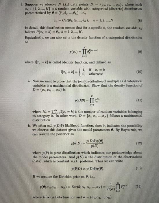
3. Suppose we observe N i.id data points D = {x,y,... In), where each 2 {1, 2, ...,K) is a random variable with categorical (discrete) distribution parameterized by 0 = (0., 8., ...,Ox), i.e., In Cat(0.02 ...,Ox), n=1,2,..., N (8) In detail, this distribution means that for a specific n, the random variable In follows P(in = k) = 0x, k=1,2,..., K. Equivalently, we can also write the density function of a categorical distribution BS plen) - LTO- where I . = k] is called identity function, and defined as 11. = 4) = { if - otherwise (10) 0, a. Now we want to prove that the joiniylistribution of multiple i.i.d categorical variables is a multinomial distribution. Show that the density function of D= {11, 12,., In} is p(D|) - II ON (11) where N = N1[In = k) is the number of random variables belonging to category k. In other word, D = {21, 12, ..., In} follows a multinomial distribution. b. We often call p(DIO) likelihood function, since it indicates the possibility we observe this dataset given the model parameters 6. By Bayes rule, we can rewrite the posterior as p( DpO) (12) P(D) where p() is piror distribution which indicates our preknowledge about the model parameters. And p(D) is the distribution of the observations (data), which is constant w.r.t. posterior. Thus we can write p(OD) p( DpO) (13) p(OD) If we assume the Dirichlet prior on i.e., K p(0:1, 42, ....ax) = Dir(6.a., 22.., ) 1 Bla (14) where Bla) is Beta function and a (Qi09) Now try to derive the joint distribution p(D, 2) and ignore the constant term w.r.t. a. Show that the posterior is actually also Dirichlet and parameterized as follows: p(OD) = Dir(0; 01 + N1,02 + N2, ..., QX + Nx) (15) [In fact, this nice property is called conjugacy in machine learning. A general statement is : If the prior distribution is conjuagate to the likelihood, then the posterior will be the same distribution as the prior distribution. Search conjugate prior and exponential family for more detail if you are interested.]