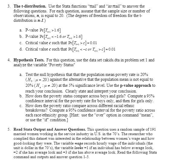
3. The t-distribution. Use the State functions "ttail" and "invitail" to answer the following questions. For each question, assume that the sample size or number of observations, m, is equal to 20. (The degrees of freedom of freedom for the t- distribution is n-1.) a. P-value Pr[7,, > 1.6] b. P-value Pr[7,,, 1.6] c. Critical value c such that Pr[7, > c] =0.01 d. Critical value c such that Pr[7, > c]=0.01 4. Hypothesis Tests. For this question, use the data set cakids.dta in problem set 1 and analyze the variable "Poverty Status" a. Test the null hypothesis that that the population mean poverty rate is 20% (Ho : u = .20) against the alternative that the population mean is not equal to 20% (H. : u = .20) at the 5% significance level. Use the p-value approach to reach your conclusion. Clearly state and interpret your conclusion. b. How does the poverty status compare across boys and girls? Compute a 95% confidence interval for the poverty rate for boys only, and then for girls only. c. How does the poverty ratio compare across different racial/ethnic breakdowns? Compute a 95% confidence interval for the poverty ratio across each race/ethnicity group. [Hint: use the "over" option in command "mean"; or use the "if" condition.] 5. Read Stata Output and Answer Questions. This question uses a random sample of 191 married women working in the service industry in U.S. in the 70's. The researcher who complied this dataset was interested in the relationship between women's wage and how good-looking they were. The variable wage records hourly wage of the individuals (the unit is dollar in the 70's), the variable looks =1 if an individual has below average look, =2 if she has average look and =3 if she has above average look. Read the following State command and outputs and answer question 1-5