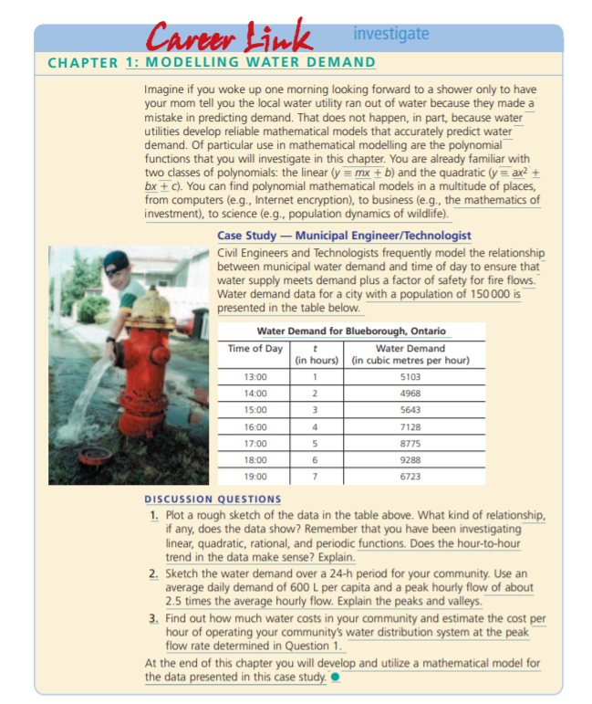
4. Using the data presented above, develop and utilize a polynomial mathematical model of the flow-rate and time relationship [Q=f (t)] by a). determining the degree of the polynomial, then using the graphing calculator to obtain an algebraic model for Q=f (t) with the appropriate polynomial regression function. b). using the graphing calculator to determine the peak flow. When does this occur? Is this a reasonable time for a peak daily flow? Explain. c). determining an algebraic model for the velocity [V(t)] of the water in the pipe (metres per hour) leaving the water plant if the cross-sectional area [A(t)] of the pipe changes over time with the relationship: A(t)=0.1t+0.4 where A(t) is cross-sectional area in square metres, t is time in hours, and Q(t)=A(t) V(t). d). verifying that your model in part c is correct using the graphing calculator. Explain how you did this.

Career Link investigate CHAPTER 1: MODELLING WATER DEMAND Imagine if you woke up one morning looking forward to a shower only to have your mom tell you the local water utility ran out of water because they made a mistake in predicting demand. That does not happen, in part, because water utilities develop reliable mathematical models that accurately predict water demand. Of particular use in mathematical modelling are the polynomial functions that you will investigate in this chapter. You are already familiar with two classes of polynomials: the linear (y = mx + b) and the quadratic (y = ax2 + bx + C). You can find polynomial mathematical models in a multitude of places, from computers (e.g., Internet encryption), to business (e.g., the mathematics of investment), to science (e.g., population dynamics of wildlife). Case Study - Municipal Engineer/Technologist Civil Engineers and Technologists frequently model the relationship between municipal water demand and time of day to ensure that water supply meets demand plus a factor of safety for fire flows. Water demand data for a city with a population of 150 000 is presented in the table below. Water Demand for Blueborough, Ontario Time of Day Water Demand (in hours) (in cubic metres per hour) 5103 13:00 14:00 1 2 4968 5643 15:00 3 16:00 4 5 17:00 18:00 19:00 7128 8775 9288 6723 6 7 DISCUSSION QUESTIONS 1. Plot a rough sketch of the data in the table above. What kind of relationship, if any, does the data show? Remember that you have been investigating linear, quadratic, rational, and periodic functions. Does the hour-to-hour trend in the data make sense? Explain. 2. Sketch the water demand over a 24-h period for your community. Use an average daily demand of 600 L per capita and a peak hourly flow of about 2.5 times the average hourly flow. Explain the peaks and valleys. 3. Find out how much water costs in your community and estimate the cost per hour of operating your community's water distribution system at the peak flow rate determined in Question 1. At the end of this chapter you will develop and utilize a mathematical model for the data presented in this case study. Career Link investigate CHAPTER 1: MODELLING WATER DEMAND Imagine if you woke up one morning looking forward to a shower only to have your mom tell you the local water utility ran out of water because they made a mistake in predicting demand. That does not happen, in part, because water utilities develop reliable mathematical models that accurately predict water demand. Of particular use in mathematical modelling are the polynomial functions that you will investigate in this chapter. You are already familiar with two classes of polynomials: the linear (y = mx + b) and the quadratic (y = ax2 + bx + C). You can find polynomial mathematical models in a multitude of places, from computers (e.g., Internet encryption), to business (e.g., the mathematics of investment), to science (e.g., population dynamics of wildlife). Case Study - Municipal Engineer/Technologist Civil Engineers and Technologists frequently model the relationship between municipal water demand and time of day to ensure that water supply meets demand plus a factor of safety for fire flows. Water demand data for a city with a population of 150 000 is presented in the table below. Water Demand for Blueborough, Ontario Time of Day Water Demand (in hours) (in cubic metres per hour) 5103 13:00 14:00 1 2 4968 5643 15:00 3 16:00 4 5 17:00 18:00 19:00 7128 8775 9288 6723 6 7 DISCUSSION QUESTIONS 1. Plot a rough sketch of the data in the table above. What kind of relationship, if any, does the data show? Remember that you have been investigating linear, quadratic, rational, and periodic functions. Does the hour-to-hour trend in the data make sense? Explain. 2. Sketch the water demand over a 24-h period for your community. Use an average daily demand of 600 L per capita and a peak hourly flow of about 2.5 times the average hourly flow. Explain the peaks and valleys. 3. Find out how much water costs in your community and estimate the cost per hour of operating your community's water distribution system at the peak flow rate determined in Question 1. At the end of this chapter you will develop and utilize a mathematical model for the data presented in this case study