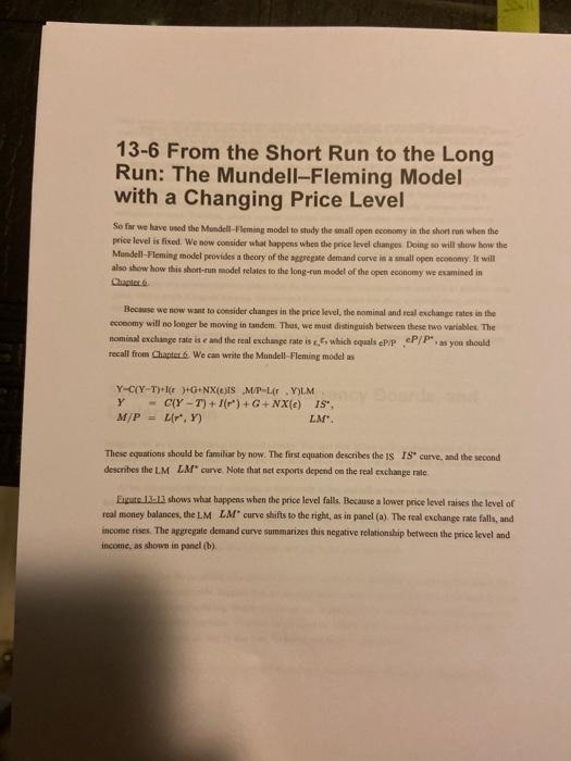
4.2. Do Mankiw, chapter 13, exercise 6. It helps to assume that the economy starts in a steady state with inflation and unemployment u", and to construct a table showing how r, un and u have to evolve through time. You may find it hard to work out what happens exactly in the long run. Don't worry too much if so- the arithmetical relation below may help. 12-1/4 + 1/8 - 1/16 + 1/32-....-1/3 13-6 From the Short Run to the Long Run: The Mundell-Fleming Model with a Changing Price Level So far we have used the Mundell-Fleming model to study the small open economy in the short run when the price level is fixed. We now consider what happens when the price level changes Doing so will show how the Mondell-Fleming model provides a theory of the pregate demand corve in a small open economy. It will also show how this short-un model relates to the long-run model of the open economy we examined in Because we now want to consider changes in the price level, the nominal and real exchange rates in the ccceomy will no longer be moving in tandem. Thus, we must distinguish between these two variable. The nominal exchange rate ise and the real exchange rate is , which equals ePvP cP/Pas you should recall from Chapter 6. We can write the Mondell-Fleming model as Y-C(Y-T)+L(r )+G+NX(e) .MP-Lr .YILM Y - ClY - 7") + (r)+G+NX(e) IS, M/P - Llr, LM". These equations should be familiar by now. The first equation describes the IS IS curve, and the second describes the LM La curve Note that net exports depend on the real exchange rate Egute 1.3.12 shows what happens when the price level falls. Because a lower price level raises the level of real money balances, the LM LM curve shifts to the right, as in panel(a). The real exchange rate falls, and income rises. The aggregate demand curve summarizes this negative relationship between the price level and income, as shown in panel (b). 4.2. Do Mankiw, chapter 13, exercise 6. It helps to assume that the economy starts in a steady state with inflation and unemployment u", and to construct a table showing how r, un and u have to evolve through time. You may find it hard to work out what happens exactly in the long run. Don't worry too much if so- the arithmetical relation below may help. 12-1/4 + 1/8 - 1/16 + 1/32-....-1/3 13-6 From the Short Run to the Long Run: The Mundell-Fleming Model with a Changing Price Level So far we have used the Mundell-Fleming model to study the small open economy in the short run when the price level is fixed. We now consider what happens when the price level changes Doing so will show how the Mondell-Fleming model provides a theory of the pregate demand corve in a small open economy. It will also show how this short-un model relates to the long-run model of the open economy we examined in Because we now want to consider changes in the price level, the nominal and real exchange rates in the ccceomy will no longer be moving in tandem. Thus, we must distinguish between these two variable. The nominal exchange rate ise and the real exchange rate is , which equals ePvP cP/Pas you should recall from Chapter 6. We can write the Mondell-Fleming model as Y-C(Y-T)+L(r )+G+NX(e) .MP-Lr .YILM Y - ClY - 7") + (r)+G+NX(e) IS, M/P - Llr, LM". These equations should be familiar by now. The first equation describes the IS IS curve, and the second describes the LM La curve Note that net exports depend on the real exchange rate Egute 1.3.12 shows what happens when the price level falls. Because a lower price level raises the level of real money balances, the LM LM curve shifts to the right, as in panel(a). The real exchange rate falls, and income rises. The aggregate demand curve summarizes this negative relationship between the price level and income, as shown in panel (b)


