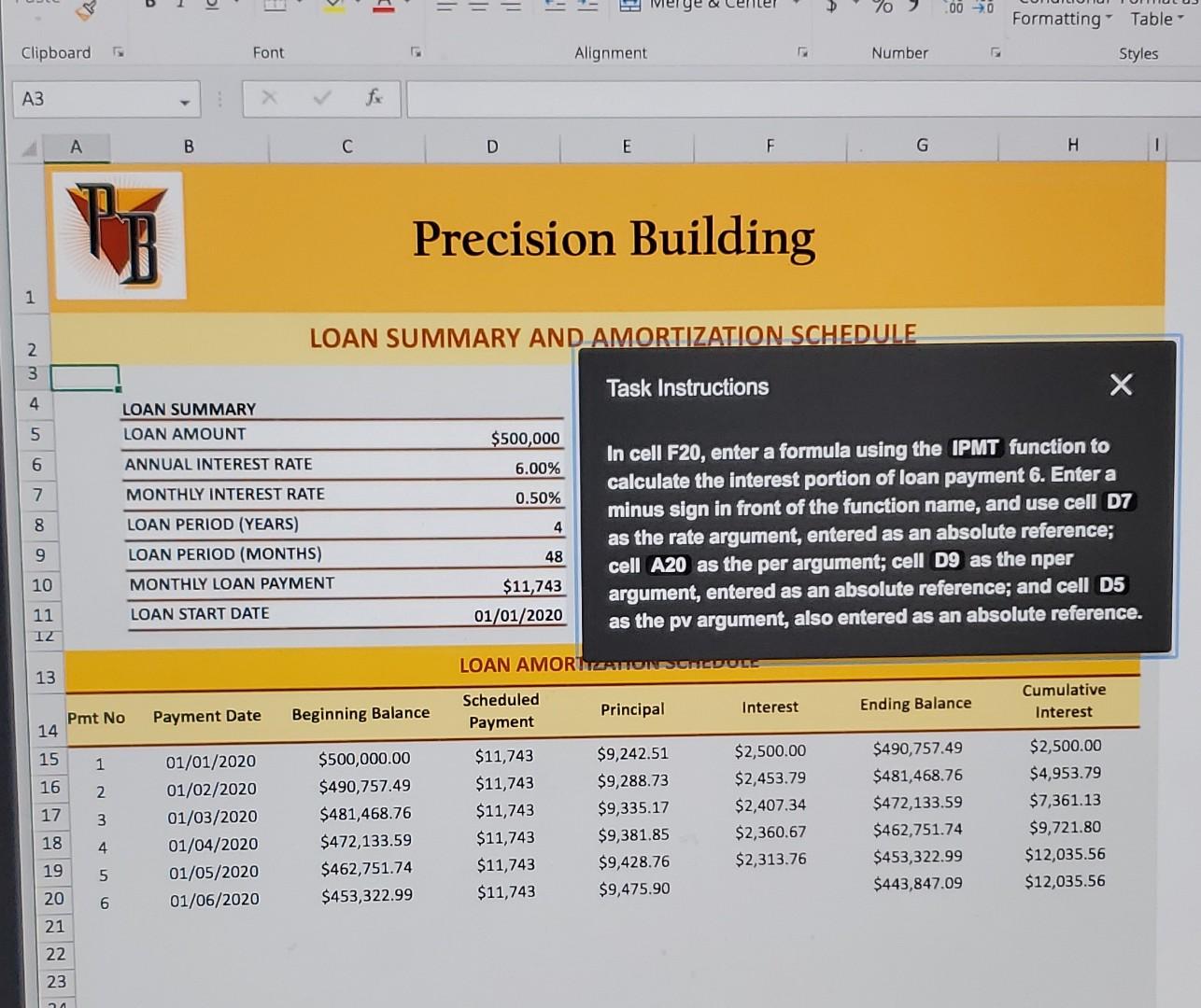
5 - 1 1 = = 70 000 Formatting Table Clipboard T Font Alignment Number Styles A3 X f B D E F G H 1 Precision Building 1 LOAN SUMMARY AND AMORTIZATION SCHEDULE 2 3 Task Instructions 4 Jou WN LOAN SUMMARY LOAN AMOUNT 5 $500,000 ANNUAL INTEREST RATE 6.00% 7 MONTHLY INTEREST RATE 0.50% 4 000 LOAN PERIOD (YEARS) LOAN PERIOD (MONTHS) In cell F20, enter a formula using the IPMT function to calculate the interest portion of loan payment 6. Enter a minus sign in front of the function name, and use cell D7 as the rate argument, entered as an absolute reference; cell A20 as the per argument; cell D9 as the nper argument, entered as an absolute reference; and cell D5 as the pv argument, also entered as an absolute reference. 48 10 MONTHLY LOAN PAYMENT $11,743 01/01/2020 LOAN START DATE 11 12 LOAN AMORTYZONUNCUOLE 13 Interest Cumulative Interest Scheduled Payment Pmt No 14 Principal Payment Date Beginning Balance Ending Balance 15 1 16 2 17 01/01/2020 01/02/2020 01/03/2020 01/04/2020 01/05/2020 01/06/2020 3 $500,000.00 $490,757.49 $481,468.76 $472,133.59 $462,751.74 $453,322.99 $11,743 $11,743 $11,743 $11,743 $11,743 $11,743 $2,500.00 $2,453.79 $2,407.34 $2,360.67 $2,313.76 $9,242.51 $9,288.73 $9,335.17 $9,381.85 $9,428.76 $9,475.90 $490,757.49 $481,468.76 $472,133.59 $462,751.74 $453,322.99 $443,847.09 $2,500.00 $4,953.79 $7,361.13 $9,721.80 $12,035.56 $12,035.56 18 4 19 5 20 6 21 22 23 5 - 1 1 = = 70 000 Formatting Table Clipboard T Font Alignment Number Styles A3 X f B D E F G H 1 Precision Building 1 LOAN SUMMARY AND AMORTIZATION SCHEDULE 2 3 Task Instructions 4 Jou WN LOAN SUMMARY LOAN AMOUNT 5 $500,000 ANNUAL INTEREST RATE 6.00% 7 MONTHLY INTEREST RATE 0.50% 4 000 LOAN PERIOD (YEARS) LOAN PERIOD (MONTHS) In cell F20, enter a formula using the IPMT function to calculate the interest portion of loan payment 6. Enter a minus sign in front of the function name, and use cell D7 as the rate argument, entered as an absolute reference; cell A20 as the per argument; cell D9 as the nper argument, entered as an absolute reference; and cell D5 as the pv argument, also entered as an absolute reference. 48 10 MONTHLY LOAN PAYMENT $11,743 01/01/2020 LOAN START DATE 11 12 LOAN AMORTYZONUNCUOLE 13 Interest Cumulative Interest Scheduled Payment Pmt No 14 Principal Payment Date Beginning Balance Ending Balance 15 1 16 2 17 01/01/2020 01/02/2020 01/03/2020 01/04/2020 01/05/2020 01/06/2020 3 $500,000.00 $490,757.49 $481,468.76 $472,133.59 $462,751.74 $453,322.99 $11,743 $11,743 $11,743 $11,743 $11,743 $11,743 $2,500.00 $2,453.79 $2,407.34 $2,360.67 $2,313.76 $9,242.51 $9,288.73 $9,335.17 $9,381.85 $9,428.76 $9,475.90 $490,757.49 $481,468.76 $472,133.59 $462,751.74 $453,322.99 $443,847.09 $2,500.00 $4,953.79 $7,361.13 $9,721.80 $12,035.56 $12,035.56 18 4 19 5 20 6 21 22 23