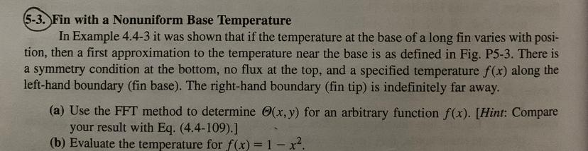
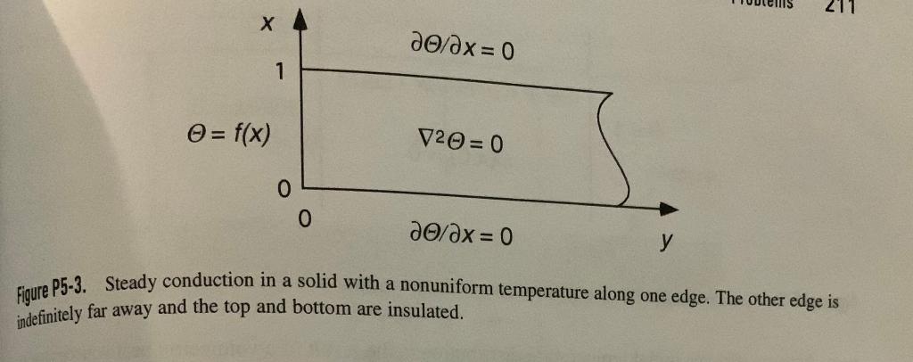
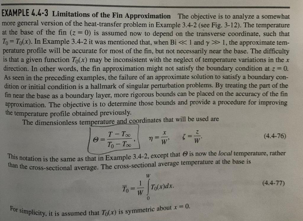
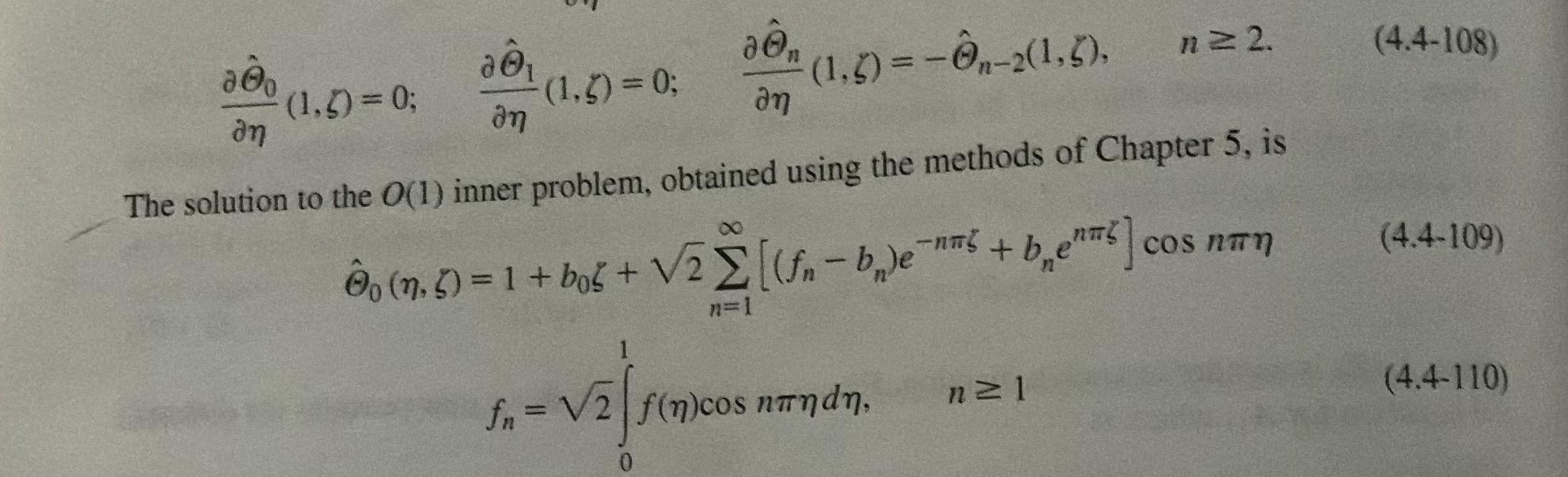
5-3. Fin with a Nonuniform Base Temperature In Example 4.4-3 it was shown that if the temperature at the base of a long fin varies with position, then a first approximation to the temperature near the base is as defined in Fig. P5-3. There is a symmetry condition at the bottom, no flux at the top, and a specified temperature f(x) along the left-hand boundary (fin base). The right-hand boundary (fin tip) is indefinitely far away. (a) Use the FFT method to determine (x,y) for an arbitrary function f(x). [Hint: Compare your result with Eq. (4.4-109).] (b) Evaluate the temperature for f(x)=1x2. Figure P5-3. Steady conduction in a solid with a nonuniform temperature along one edge. The other edge is indefinitely far away and the top and bottom are insulated. EXAMPLE 4.4-3 Limitations of the Fin Approximation The objective is to analyze a somewhat more general version of the heat-transfer problem in Example 3.4-2 (see Fig. 3-12). The temperature at the base of the fin (z=0) is assumed now to depend on the transverse coordinate, such that T0=T0(x). In Example 3.4-2 it was mentioned that, when Bi1 and 1, the approximate temperature profile will be accurate for most of the fin, but not necessarily near the base. The difficulty is that a given function T0(x) may be inconsistent with the neglect of temperature variations in the x direction. In other words, the fin approximation might not satisfy the boundary condition at z=0. As seen in the preceding examples, the failure of an approximate solution to satisfy a boundary condition or initial condition is a hallmark of singular perturbation problems. By treating the part of the fin near the base as a boundary layer, more rigorous bounds can be placed on the accuracy of the fin approximation. The objective is to determine those bounds and provide a procedure for improving the temperature profile obtained previously. The dimensionless temperature and coordinates that will be used are =T0TTT,=Wx,=Wz. This notation is the same as that in Example 3.4-2, except that is now the local temperature, rather than the cross-sectional average. The cross-sectional average temperature at the base is T0=W10WT0(x)dx For simplicity, it is assumed that T0(x) is symmetric about x=0. ^0(1,)=0;^1(1,)=0;^n(1,)=^n2(1,),n2 The solution to the O(1) inner problem, obtained using the methods of Chapter 5 , is ^0(,)=1+b0+2n=1[(fnbn)en+bnen]cosn fn=201f()cosnd,n1 The scaling used for the inner region assumes that 1 there, or that the inner region has a dimensional thickness of W. This may be checked by examining the infinite series in Eq. (4.4-114) because that is the largest term that distinguishes the inner and outer solutions. The most slowly decaying term in the sum, e, is already quite small for =1, which is consistent with the scaling assumption. This illustrates a point mentioned in Section 3.4, which is that edge effects in conduction and diffusion are important over only about one thickness of the region being modeled. That is, deviations from the fin approximation near the base are a type of edge effect