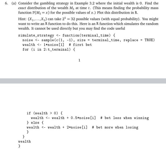
6. (a) Consider the gambling strategy in Example 3.2 where the initial wealth is 0. Find the

exact distribution of the wealth M5 at time t. (This means finding the probability mass

function P(M5 = x) for the possible values of x.) Plot this distribution in R.

Hint: (X1, . . . , X5) can take 25 = 32 possible values (with equal probability). You might

want to write an R function to do this. Here is an R function which simulates the random

wealth. It cannot be used directly but you may find the code useful

simulate_strategy

noise

wealth

for (i in 2:t_terminal) {

if (wealth > 0) {

wealth

} else {

wealth

}

}

wealth

}

(b) Define the following gambling strategy in the context of Section 3.1: For the first two

rounds bet 1 = 2 = 2. Before deciding the bet t for round t 3, consider the results

of the previous two bets. If we won both two bets, bet t = 5. If we won only one bet,

bet t = 0.5. If we lost both bets, bet t = 1. (By convention, we say that we won a

bet if the corresponding change of wealth Ms Ms1 is positive.)

Write an R function simulates computes the wealth MT (with M0 = 0):

mywealth

... # implementation

}

Sample N = 10000 paths and plot the empirical distribution of M10. (Something like the

blue part of Figure 3.1. But plot the graph in the usual way.)

6. (a) Consider the gambling strategy in Example 3.2 where the initial wealth is 0. Find the exact distribution of the wealth M, at time t. (This means finding the probability mass function P(M = x) for the possible values of x.) Plot this distribution in R. Hint: (X1,...,x) can take 25 = 32 possible values (with equal probability). You might want to write an R function to do this. Here is an R function which simulates the random wealth. It cannot be used directly but you may find the code useful simulate_strategy 0) { wealth 0, we bet Et+1 = 0.5, and otherwise we bet Et+1 = 2. The idea behind this strategy is that we bet less when we are winning, and more when we are losing. Note that t+1 is a function of M, which is in turn a function of X1,...,X In Figure 3.1 we plot the distribution of M10 if the initial wealth is Mo = 0. Note that the distribution is highly skewed towards the left. By varying the gambling strategy, we can generate a wide variety of distributions. However, as a consequence of Proposition 3.1 the expected value of Mo must be 0. 6. (a) Consider the gambling strategy in Example 3.2 where the initial wealth is 0. Find the exact distribution of the wealth M, at time t. (This means finding the probability mass function P(M = x) for the possible values of x.) Plot this distribution in R. Hint: (X1,...,x) can take 25 = 32 possible values (with equal probability). You might want to write an R function to do this. Here is an R function which simulates the random wealth. It cannot be used directly but you may find the code useful simulate_strategy 0) { wealth 0, we bet Et+1 = 0.5, and otherwise we bet Et+1 = 2. The idea behind this strategy is that we bet less when we are winning, and more when we are losing. Note that t+1 is a function of M, which is in turn a function of X1,...,X In Figure 3.1 we plot the distribution of M10 if the initial wealth is Mo = 0. Note that the distribution is highly skewed towards the left. By varying the gambling strategy, we can generate a wide variety of distributions. However, as a consequence of Proposition 3.1 the expected value of Mo must be 0